In-Depth Classical Electromagnetism
This page is print-friendly. Simply press Ctrl + P (or Command + P if you use a Mac) to print the page and download it as a PDF. Report an issue or error here.
Table of contents
Note: it is highly recommended to navigate by clicking links in the table of contents! It means you can use the back button in your browser to go back to any section you were reading, so you can jump back and forth between sections!
- Introduction to classical electromagnetism
- Gauss's law
- Electric potential
- Solving Poisson's equation
- Fields of polarized dielectrics
- Magnetostatics
- Ampère's law
- The magnetic vector potential
- Magnetic fields inside matter
- Electromagnetic induction
- Maxwell's equations and electrodynamics
- Relativistic electrodynamics
- Concluding thoughts
This is a guide to classical electromagnetism beyond the basics, tackling boundary-value problems in electrostatics and magnetostatics, electric and magnetic fields within materials, and relativistic electrodynamics.
I thank Professor Persans at Rensselaer Polytechnic Institute, without whom this guide would not have been possible.
Introduction to classical electromagnetism
Classical electromagnetism concerns the study of electrical and magnetic phenomena. It postulates that electricity and magnetism are phenomena that may be modelled using notions of charge, current, and fields. Charge is a fundamental property of objects that gives rise to electricity and magnetism; current is the flow of charge; and fields are physical quantities that span space and transmit interactions between objects (which, in this case, are charged objects).
In classical electromagnetism, there exists an electromagnetic field, with electrical and magnetic components that form one singular field. For mathematical convenience, we may separately analyze the electric components as a electric field and the magnetic components as a magnetic fields. We represent the electric field using a vector-valued function $\mathbf{E}(\mathbf{r}, t)$ and the magnetic field using a vector-valued function $\mathbf{B}(\mathbf{r}, t)$.
Units are a fundamental part of describing electromagnetic phenomena. The units used in this guide are the SI units system, also called MKS(A) units (which stands for meter-kilogram-second-ampere). The following SI units are a short list of those commonly used in electromagnetic theory:
| Unit | Symbol | Used for |
|---|---|---|
| Ampere | $\pu{A}$ | Electric current |
| Coulomb | $\pu{C}$ | Electric charge |
| Tesla | $\pu{T}$ | Magnetic field strength |
| Weber | $\pu{Wb}$ | Magnetic flux |
| Newton | $\pu{N}$ | Electric/magnetic force |
| Henry | $\pu{H}$ | Inductance |
| Kilogram | $\pu{kg}$ | Mass |
| Hertz | $\pu{Hz}$ | Frequency |
| Ohm | $\Omega$ | Resistance |
| Volt | $\pu{V}$ | Potential difference |
| Joule | $\pu{J}$ | Energy |
| Watt | $\pu{W}$ | Power |
Note: Alternate units used in theoretical physics are Gaussian units, Lorentz-Heaviside units, and natural units. These simplify many equations in electromagnetic theory, at the cost of being much more unfamiliar and far less used in daily life.
Note that a lot of this guide follows the excellent textbook by David Griffiths, Introduction to Electrodynamics (although this guide is not affiliated with Griffiths). It is highly-recommended to purchase a copy of the book as additional supplementary material to follow along with the course.
Mathematical prerequisites
The primary mathematics used in electromagnetics is vector calculus, the calculus of vectors and vector-valued functions in 3D space. We additionally use some harmonic (Fourier) analysis and infinite series, and also some special functions; we will quickly review all of these. Towards the end, we will encounter special relativity and tensor calculus, but the mathematics of tensors will be explained when we reach that section.
Note: this is not intended to be a complete review of all the mathematics involved (and is extremely fast-paced, which may not be ideal for first-time learners unfamiliar with the material). For a more extensive review on vector calculus, we suggest consulting the multivariable calculus or vector calculus guides, or read through the introductory electromagnetic theory notes.
Consider a function of a single variable $f(x)$. Then the ordinary derivative of the function is given by:
$$ \frac{df}{dx} $$
Now consider a function of multiple variables $f(x, y, z)$. Since the function has multiple inputs, the function changes at a different rate when each input is varied. Therefore, the function has more than a single derivative. We term each derivative a partial derivative, denoted:
$$ \frac{\partial f}{\partial x}, \frac{\partial f}{\partial y}, \frac{\partial f}{\partial z} $$
To compute the partial derivatives, we imagine that any variable other than the variable that is differentiated with respect to is a constant, and we can factor them out. For example:
$$ \frac{\partial}{\partial x} (3x^2 y) = 3y \frac{\partial}{\partial x} x^2 = 6xy $$
Of course, we can take higher derivatives too, such as:
$$ \frac{\partial^2 f}{\partial x^2} = \frac{\partial}{\partial x} \left(\frac{\partial f}{\partial x}\right) $$
We can also define other types of derivatives for multivariable functions. For instance, we can collect all the partial derivatives together into a vector, which we call the gradient and we denote with the symbol $\nabla$:
$$ \nabla f = \left\langle \frac{\partial f}{\partial x}, \frac{\partial f}{\partial y}, \frac{\partial f}{\partial z}\right\rangle = \frac{\partial f}{\partial \mathbf{r}} \hat r $$
A multivariable function can be one that returns a vector instead of a number. Such a function would be denoted $\mathbf{F}(x, y, z) = \langle F_x, F_y, F_z\rangle$. Then we can define a vector derivative called the divergence, represented with the same $\nabla$ symbol with a dot:
$$ \operatorname{div} \mathbf{F} = \nabla \cdot \mathbf{F} = \frac{\partial F_x}{\partial x} + \frac{\partial F_y}{\partial y} + \frac{\partial F_z}{\partial z} $$
Similarly, we can define a vector derivative called the curl, represented with the $\nabla \times$ symbol:
$$ \operatorname{curl} \mathbf{F} = \nabla \times \mathbf{F} = \left \langle \frac{\partial F_z}{\partial y} - \frac{\partial F_y}{\partial z}, \frac{\partial F_x}{\partial z} - \frac{\partial F_z}{\partial x}, \frac{\partial F_y}{\partial x} - \frac{\partial F_x}{\partial y}\right \rangle $$
The notations for the divergence and curl are inspired by the notations for the vector dot and cross products; these become exact when, just like we can represent the differentiation operator with $\displaystyle \frac{d}{dx}$, we can represent the multivariable differentiation operator (also called the nabla operator) with:
$$ \nabla = \left\langle \frac{\partial}{\partial x}, \frac{\partial}{\partial y}, \frac{\partial}{\partial z} \right\rangle $$
With this "vector", applying the dot product and cross product formulas using $\nabla$ becomes the divergence and the curl, respectively. Finally, we have the Laplacian ("multivariable second derivative") which is given by the divergence of the curl and denoted $\nabla^2$:
$$ \nabla^2 f = \nabla \cdot \nabla f = \frac{\partial^2 f}{\partial x^2} + \frac{\partial^2 f}{\partial y^2} + \frac{\partial^2 f}{\partial z^2} $$
Multivariable integration is very similar to a partial derivative, the idea is that we separate a multivariable integral into partial integrals, where integrate only with respect to one variable at a time for each individual integral. For instance, a 3D integral might be something like:
$$ \int f(x, y, z)~dV = \iiint f(x, y, z)~dx~dy~dz $$
Here the way we solved it was to expand the integral as three individual integrals, one each for $x, y, z$. Then we do each of the integrals one by one, integrating just one variable at a time and treating all the other variables as constant:
$$ \int \left[\int \left[\int f(x, y, z) dx\right] dy\right] dz $$
There are several different types of multivariable integrals: line integrals, which are single integrals over a path, surface integrals, which are double integrals over surfaces, and volume integrals, which are triple integrals over space. It sometimes is easiest by rewriting these integrals in terms of an integration element, just like $dV = dx~dy~dz$ for volume integrals or $dA = dx~dy$ for surface integrals or $d\ell = dx \hat i + dy \hat j + dz \hat k$ for line integrals, then expand, then solve via partial integration. While this is mathematically completely non-rigorous, the physics works out just fine. Also, note that sometimes, we add a circular loop around the integral sign - this means whatever is integrated over is closed, such a closed loop for line integrals or a closed surface for surface integrals:
$$ \begin{align*} \oint \mathbf{F} \cdot d\mathbf{r} \\ \oint \mathbf{B} \cdot d\mathbf{A} \end{align*} $$
Curvilinear coordinate systems
We find that when solving some problems in electromagnetism, it is easier to use a non-Cartesian coordinate system, such as polar, cylindrical, and spherical coordinates. This is especially the case if the problem is rotationally symmetric. We illustrate the three most common non-Cartesian coordinate systems below: polar coordinates, cylindrical coordinates, and spherical coordinates.

Polar coordinates use $(r, \theta)$ to describe the location of a point, where $r$ is the radial distance from the origin to the point, and $\theta$ is the angle the point makes with the $x$ axis. Polar coordinates are related to Cartesian coordinates by:
$$ \begin{align*} x = r \cos \theta \\ y = r \sin \theta \end{align*} $$
Cylindrical coordinates extend the polar coordinate system into 3D space. It uses the coordinates $(\rho, \phi, z)$ to describe the location of a point, where $\rho$ and $\phi$ describe the point's location along the $xy$ plane, and $z$ describes the point's elevation above the $xy$ plane (you may also sometimes see the coordinates written as $(r, \theta, z)$ or $(r, \phi, z)$ but I prefer this form since it allows using the same $\phi$ as in spherical coordinates, as we'll soon see). The conversion from cylindrical coordinates to polar coordinates are given by:
$$ \begin{align*} x &= \rho \cos \phi \\ y &= \rho \sin \phi \\ z &= z \end{align*} $$
Finally, spherical coordinates describe the location of a point with coordinates $(r, \theta, \phi)$, where $r$ is the absolute distance from the point to the origin, $\theta$ is the angle of elevation the point makes with the $xy$ plane, and $\phi$ is the same (rotational) angle as the $\phi$ in cylindrical coordinates. The conversions from spherical coordinates to Cartesian are given by:
$$ \begin{align*} x &= r \sin \theta \cos \phi \\ y &= r \sin \theta \sin \phi \\ z &= r \cos \theta \end{align*} $$
The Dirac delta and Kronecker delta
In addition to vector calculus, classical electromagnetism also uses two special "functions" - the Kronecker Delta and Dirac Delta. These are technically speaking not functions, but in many ways they are similar to functions and (specifically in the case of the Dirac delta) can be treated like a function.
The Kronecker delta is written $\delta_{mn}$, where:
$$ \delta_{mn} = \begin{cases} 0, & m \neq n \\ 1, & m = n \end{cases} $$
The Kronecker Delta is very useful in expressing orthogonality. Orthogonality may be more familiar when discussed using vectors; two unit vectors have a dot product of zero when they are parallel (and thus equal to each other) and one when they are orthogonal (perpendicular to each other). However, we may generalize this principle for functions. The orthogonality relations for the sine function, for instance, are given by:
$$ \begin{align*} \int_{-\ell}^\ell \sin \left(\dfrac{m\pi x}{\ell}\right) \sin \left(\dfrac{n\pi x}{\ell}\right)\,dx &= \ell \delta_{mn} = \begin{cases} \ell ,& m = n \\ 0, & m \neq n \end{cases} \\ \int_{0}^\ell \sin \left(\dfrac{m\pi x}{\ell}\right) \sin \left(\dfrac{n\pi x}{\ell}\right)\,dx &= \dfrac{\ell}{2} \delta_{mn} = \begin{cases} \ell/2 ,& m = n \\ 0, & m \neq n \end{cases} \end{align*} $$
And for the cosine function, we have:
$$ \int_{0}^\ell \cos \left(\dfrac{m\pi x}{\ell}\right) \cos \left(\dfrac{n\pi x}{\ell}\right)\,dx = \dfrac{\ell}{2} \delta_{mn} = \begin{cases} \ell/2 ,& m = n, & m, n \neq 0 \\ \ell, & m = n = 0 \\ 0, & m \neq n \end{cases} $$
The Dirac delta is a generalization of the Kronecker delta (which takes a binary discrete input) for continuous inputs. It is defined by:
$$ \delta(x) = \begin{cases} 0, & x \neq 0 \\ 1, & x = 0 \end{cases} $$
Note: the Dirac delta can be thought of as a function that looks like a "spike" at $x = 0$ and is zero everywhere else.
The Dirac delta's usefulness mostly comes from the fact that it possesses a very special integral:
$$ \int_a^b \delta(x)\, dx = 1 $$
Which also means that if the Dirac delta were displaced by a certain amount $x'$, then assuming $a < x' < b$:
$$ \begin{align*} \int_a^b f(x)\delta(x- x')dx &= f(x') \\ \int_a^b f(x')\delta(x-x')dx &= f(x) \end{align*} $$
This is incredibly useful (as we'll see) for describing quantities that exist only at one point in space (e.g. a point charge, which has the charge density $\rho(\mathbf{r}) = Q\delta(\mathbf{r}-\mathbf{r}')$).
Note that the Dirac delta can also be generalized to 2D (where it is written $\delta^2(\mathbf{r} - \mathbf{r}')$) and 3D (where it is written $\delta^3(\mathbf{r} - \mathbf{r}')$. The following expressions are for the 2D Dirac delta expressed in Cartesian and polar coordinates:
| Coordinate system | Expression for Dirac Delta "function" |
|---|---|
| Cartesian $(x, y)$ | $\delta^2(\mathbf{r} - \mathbf{r}') = \delta(x - x')\delta(y-y')$ |
| Polar $(r, \theta)$ | $\delta^2(\mathbf{r} - \mathbf{r}') = \dfrac{1}{r}\delta(r-r')\delta(\theta-\theta')$ |
And the following expressions are for the 3D Dirac delta $\delta^3(\mathbf{r} - \mathbf{r}')$ in Cartesian, cylindrical, and spherical coordinates:
| Coordinate system | Expression for Dirac Delta "function" |
|---|---|
| Cartesian $(x, y, z)$ | $\delta^3(\mathbf{r} - \mathbf{r}') = \delta(x-x')\delta(y-y')\delta(z-z')$ |
| Cylindrical $(\rho, \phi, z)$ | $\delta^3(\mathbf{r} - \mathbf{r}') = \dfrac{1}{\rho}\delta (\rho - \rho')\delta(\phi-\phi')\delta(z-z')$ |
| Spherical $(r, \theta, \phi)$ | $\delta^3(\mathbf{r} - \mathbf{r}') = \dfrac{1}{r^2 \sin \theta} \delta(r - r') \delta(\theta - \theta') \delta(\phi - \phi')$ |
We have now completed our short review of the essential mathematics for studying electromagnetism. Again, see the dedicated resources in the calculus series for a slower-paced, more detailed guide to all of these topics. But for the purposes of this guide, we will now move on to the exciting part - the physics of electromagnetism.
Review of Maxwell's equations
In introductory electromagnetic theory, we have found that the fundamental laws of electromagnetism are Maxwell's equations, a series of four coupled partial differential equations that describe the electric and magnetic fields:
| Equation name | Integral form | Differential form |
|---|---|---|
| Gauss's law for electricity | $\displaystyle \oint \mathbf{E} \cdot d\mathbf{A} = \dfrac{1}{\varepsilon_0} \int \rho, dV$ | $\nabla \cdot \mathbf{E} = \rho/\varepsilon_0$ |
| Gauss's law for magnetism | $\displaystyle \oint \mathbf{B} \cdot d\mathbf{A} = 0$ | $\nabla \cdot \mathbf{B} = 0$ |
| Faraday's law | $\displaystyle \oint \mathbf{E}\cdot d\mathbf{r} = -\dfrac{d}{dt} \displaystyle \iint \mathbf{E} \cdot d\mathbf{A}$ | $\nabla \cdot \mathbf{E} = -\dfrac{\partial \mathbf{B}}{\partial t}$ |
| Ampere-Maxwell law | $\displaystyle \oint \mathbf{B} \cdot d\mathbf{r} = \mu_0 \iint \mathbf{J} \cdot d\mathbf{A} + \mu_0 \varepsilon_0 \dfrac{d}{dt} \displaystyle \iint \mathbf{B} \cdot d\mathbf{A}$ | $\nabla \cdot \mathbf{B} = \mu_0 \mathbf{J} + \mu_0 \varepsilon_0 \dfrac{\partial \mathbf{E}}{\partial t}$ |
We also found that light is an electromagnetic phenomenon, and that the speed of light $c$ in vacuum can be expressed in terms of the electric constant $\varepsilon_0$ and the magnetic constant $\mu_0$ as:
$$ c = \dfrac{1}{\sqrt{\mu_0 \varepsilon_0}} $$
Note: the speed of light will be different inside of materials; it is only its speed in vacuum that is constant and takes the value of $c$. For instance, light passes about 33% slower through glass and 58% slower through diamond, and significantly slowly in materials cooled to almost absolute zero. However, the vacuum speed of light is a universal constant and stringent experimental tests have found no difference in the vacuum speed of light in a variety of different conditions.
Finally, we found that the equations of motion of a charged particle in an electromagnetic field follow the Lorentz force law $m\ddot {\mathbf{r}} = q(\mathbf{E} + \mathbf{v} \times \mathbf{B})$, formed by a combination of the electric force $\mathbf{F}_E = q\mathbf{E}$ and the magnetic force $\mathbf{F}_B = q\mathbf{v} \times \mathbf{B}$. In the special case where charged particles are moving at a significant fractional of the speed of light, they follow the relativistic version of the same law:
$$ \dfrac{d}{dt}\left(\dfrac{mv}{\sqrt{1 - (v/c)^2}}\right) = q(\mathbf{E} + \mathbf{v} \times \mathbf{B}) $$
Review of electrostatics
Previously in introductory electromagnetic theory, we discussed the concepts of electric force and electric field in electrostatic scenarios. Electrostatics governs the behavior of slow-moving and stationary charges. The electric force exerted by charge $q_1$ on charge $q_2$ (pay attention to the order) is given by Coulomb's law:
$$ \mathbf{F}_\text{1 on 2} = \dfrac{k q_1 q_2}{|\mathbf{r}_2 - \mathbf{r}_1|^3} (\mathbf{r}_2 - \mathbf{r}_1) $$
Where $\mathbf{r}_2 - \mathbf{r}_1$ is the displacement vector between the positions of the charges, and points from $q_1$ to $q_2$. For $n$ charges, the electric force is the sum of all the individual electric forces:
$$ \mathbf{F}_\mathrm{total} = \mathbf{F}_\text{1 on 2} + \mathbf{F}_\text{3 on 2} + \mathbf{F}_\text{4 on 2} + \dots + \mathbf{F}_{n\ \text{on 2}} $$
Note: You may wonder why the denominator of Coulomb's law contains a cubed term when the electric force is known to be an inverse-square law. The answer is more apparent if we rewrite Coulomb's law in terms of a unit vector $\hat r_{12} = \dfrac{\mathbf{r}_2 - \mathbf{r}_1}{|\mathbf{r}_2 - \mathbf{r}_1|}$, for which Coulomb's law can be written as $\mathbf{F}_\text{1 on 2} = \dfrac{kq_1 q_2}{|\mathbf{r}_2 - \mathbf{r}_1|} \hat r_{12}$ which translates to $\mathbf{F}_\text{1 on 2} = \dfrac{kq_1 q_2}{|\mathbf{r}_2 - \mathbf{r}_1|} \dfrac{\mathbf{r}_2 - \mathbf{r}_1}{|\mathbf{r}_2 - \mathbf{r}_1|} = \dfrac{k q_1 q_2}{|\mathbf{r}_2 - \mathbf{r}_1|^3} (\mathbf{r}_2 - \mathbf{r}_1)$.
Calculating electric forces may seem deceptively simple, but for large numbers of charges it becomes very challenging due to the large number of inter-charge forces. It is much easier to instead calculate an electric field, and use the electric force law $\mathbf{F}_E = q\mathbf{E}$ to calculate the total electric force on a charge due to all the other charges. The electric field of a single point charge located at the origin is given by:
$$ \mathbf{E} = \dfrac{kQ}{r^2} \hat r $$
The more general expression for the electric field $\mathbf{E}(\mathbf{r}) = \mathbf{E}(x, y, z)$ formed by $N$ charges, of which each charge $Q_i$ is situated at position $\mathbf{r}_i$, is given by:
$$ \mathbf{E}(\mathbf{r}) = \sum \limits_{i = 1}^N \dfrac{kQ_i}{|\mathbf{r} - \mathbf{r}_i|^3}(\mathbf{r} - \mathbf{r}_i) $$
It may prove useful to explicitly write out the expression in Cartesian coordinates. Then the electric field may be written:
$$ \mathbf{E}(x, y, z) = \sum \limits_{i = 1}^N \dfrac{kQ_i[(x - x_i)\hat i + (y - y_i)\hat j + (z - z_i)\hat k]}{[(x - x_i)^2 + (y - y_i)^2 + (z - z_i)^2]^\frac{3}{2}} $$
In the continuous case, where we have a charge distribution such as $\lambda(x)$ (linear charge density), $\sigma(x, y)$ (surface charge density), or $\rho(x, y, z)$ (volume charge density), then:
$$ \mathbf{E}(\mathbf{r}) = \int \dfrac{k dq'}{|\mathbf{r} - \mathbf{r}'|^3} (\mathbf{r} - \mathbf{r}') $$
Where $\mathbf{r}'$ is the location of infinitesimal charge element $dq'$, and $\mathbf{r} - \mathbf{r}'$ is the displacement vector. For linear, surface, and volume charge distributions, we have respectively $dq' = \lambda ds' = \sigma dA' = \rho dV'$ so the integral becomes:
$$ \begin{align*} \mathbf{E}(\mathbf{r}) &= \int_C k\dfrac{\lambda ds'}{|\mathbf{r} - \mathbf{r}'|^3} (\mathbf{r} - \mathbf{r}'), &\text{(linear charge)} \\ &= \int_S k\dfrac{\sigma dx'dy'}{|\mathbf{r} - \mathbf{r}'|^3} (\mathbf{r} - \mathbf{r}'), &\text{(surface charge)} \\ &= \int_V k\dfrac{\sigma dx'dy'dz'}{|\mathbf{r} - \mathbf{r}'|^3} (\mathbf{r} - \mathbf{r}'), &\text{(volume charge)} \end{align*} $$
Note: be careful to remember that the integration is over $x', y', z'$, not $x, y, z$! Therefore, the final integral should have the integration variables $dx', dy', dz'$ and bounds in $x', y', z'$. In some cases, it may be possible to express $x', y', z$ purely in terms of $x, y, z$, and similarly express $dx', dy', dz'$ in terms of $dx, dy, dz$; when all variables involving $x', y', z'$ are eliminated and replaced with $x, y, z$, then indeed it is possible to simply integrate over $x, y, z$. This, however, is not true in the general case.
Gauss's law
In the previous section, we covered the discrete and integral forms of Coulomb's law for electric fields. This method of computing the electric field is error-prone, difficult to do by hand, and inelegant, which is why it is often termed the "brute-force method". The more elegant alternative is to use Gauss's law for electric fields:
$$ \Phi_E = \oint \mathbf{E} \cdot d\mathbf{A} = \dfrac{Q_\text{total}}{\varepsilon_0} $$
Gauss's law relates the flux of the electric field $\Phi_E$, which is the surface integral of the electric field over a closed surface (called a Gaussian surface), to the total charge contained within the surface. The surface integral is defined as the integral of the field in the direction normal to the surface, that is, $\mathbf{E} \cdot d\mathbf{A} = \mathbf{E} \cdot \mathbf{n}, dA$.
The advantage of using Gauss's law is that many charge configurations exhibit certain symmetries for which the electric field is uniform across the surface:
$$ \oint \mathbf{E} \cdot d\mathbf{A} = E \oint dA $$
This makes it possible to solve for the electric field rather straightforwardly. In fact, a direct application of Gauss's law allows deriving Coulomb's law giving the electric field of a point charge at the origin. We need only choose our closed surface to be a sphere of radius $r$. As the electric field vectors are directly perpendicular to the surface, it can be factored out of the integral, such that:
$$ \oint \mathbf{E} \cdot d\mathbf{A} = E \oint dA = E(4\pi r^2) = \dfrac{Q}{\varepsilon_0} $$
Then rearrangement gives:
$$ E = \dfrac{1}{4\pi \epsilon_0} \dfrac{Q}{r^2} $$
Noting that the electric field points radially outwards for $Q > 0$ the vector form is straightforward to find:
$$ \mathbf{E} = \dfrac{1}{4\pi \epsilon_0} \dfrac{Q}{r^2}\hat r $$
And thus we have recovered the vector form of Coulomb's law, as would be expected. Note that using $k \equiv \dfrac{1}{4\pi \varepsilon_0}$ is common to be able to simplify the expression.
Notes on Gaussian surfaces
Gauss's law requires surface integration over a closed surface called a Gaussian surface. The surface normal is always chosen to be the outward-pointing normal of the surface. In many cases, the normal can be found without explicit calculation by simply analyzing the symmetries of the problem - for instance, in our spherical configuration, which possesses radial symmetry, the surface normals are given by $\hat{\mathbf{n}} = \hat r$.
In some other cases, we must explicitly find the normal vector from the surface. From multivariable calculus, given a surface implicitly-defined as $F(x, y, z) = 0$, the normal vector is given by:
$$ \hat{\mathbf{n}} = \dfrac{\nabla F}{|\nabla F|} $$
A sphere, for instance, is a surface defined by the implicit equation $F(x, y, z) = x^2 + y^2 + z^2 - R^2 = 0$, where $R$ is a constant. Therefore, $\nabla F = \langle 2x, 2y, 2y \rangle = 2 \mathbf{r}$ which has a magnitude of $2\sqrt{x^2 + y^2 + z^2} = 2|\mathbf{r}|$, so:
$$ \hat{\mathbf{n}} = \dfrac{2\mathbf{r}}{2|\mathbf{r}|} = \dfrac{\mathbf{r}}{|\mathbf{r}|} = \hat r $$
.Common solutions for electric fields from Gauss's law
The majority of electric fields cannot be solved analytically by using Gauss's law. However, analytical solutions for the field do exist for some simple geometries. Using Gauss's law, solutions to the field for several common physical scenarios are shown below:
| Physical situation | Gaussian surface | Result from flux integral | Enclosed charge | Electric field |
|---|---|---|---|---|
| Anywhere around a point charge | Sphere of radius $r$ centered at $r = 0$ | $\Phi_E = 4\pi r^2 |\mathbf{E}|$ | $Q = Q$ | $\mathbf{E} = \dfrac{1}{4\pi \varepsilon_0} \dfrac{Q}{r^2} \hat{\mathbf{r}}$ |
| Outside uniform sphere of charge with radius $R$ | Sphere of radius $r$ centered at $r = 0$ | $\Phi_E = 4\pi r^2 |\mathbf{E}|$ | $Q = Q$ | $\mathbf{E} = \dfrac{1}{4\pi \varepsilon_0} \dfrac{Q}{r^2} \hat{\mathbf{r}}, \quad r > R$ |
| Above surface of a conductor (of arbitrary thickness/geometry) | Box parallel to the surface with rectangular tops/bottoms of area $A$, placed at $z = 0$ | $\Phi_E = |\mathbf{E}|A$ | $Q = \sigma A$ | $\mathbf{E} = \dfrac{\sigma}{\varepsilon_0} \hat{\mathbf{n}}$ where $\hat{\mathbf{n}}$ is the normal vector to the conductor's surface |
| Above a single-sided infinite sheet of charge | Box with rectangular tops/bottoms of area $A$, placed at $z = 0$ | $\Phi_E = |\mathbf{E}|A$ | $Q = \sigma A$ | $\mathbf{E} = \dfrac{\sigma}{\varepsilon_0} \hat{\mathbf{z}}, \quad z > 0$ |
| Above (or below) a double-sided infinite sheet of charge | Box with rectangular tops/bottoms of area $A$ centered at $z = 0$ (i.e. it is halfway above and halfway below the sheet of charge) | $\Phi_E = 2|\mathbf{E}|A$ (flux contribution from both the top and bottom side of the Gaussian surface) | $Q = \sigma A$ | $\mathbf{E} = \dfrac{\sigma}{2\varepsilon_0} \hat{\mathbf{z}}, \quad |z| > 0$ |
| Around infinite line of charge (e.g. infinitely long wire) with charge density $\lambda$ | Coaxial cylinder (aligned along same axis as line of charge) of radius $\rho$ and length $L$ | $\Phi_E = 2\pi r L \lambda$ | $Q = \lambda L$ | $\mathbf{E} = \dfrac{\lambda}{2\pi \rho \varepsilon_0} \hat{\rho}$ (here $\rho$ is distance from wire) |
Note: An interesting consequence of Gauss's law that an infinitely-long uniformly-charged wire would have the same amount of charge regardless of its thickness. In fact, it doesn't even matter if you are inside the wire! The reason why is that their total charge $Q = \lambda L$ is independent of the thickness of the wire and also independent of the radial distance. Why? Because any infinite wire would have infinite length, and thus infinite charge, no matter its thickness, so the total charge of any infinite wire (regardless of thickness) is $\infty$, so the same! Of course, in actual calculations with real wires, we would set $L$ to a large but non-infinite value, and thus the solution would only be an approximate solution (because the electric field of real wires does depend on their thickness). But in the limit of infinite length, all wires and cylindrical charges with a uniform linear charge density $\lambda$ always have the same total charge.
Electric potential
Previously, we saw that we could express the motion of charged particles within electric fields by using the electric force law $\mathbf{F}_E = q\mathbf{E}$ as well as Coulomb's law for determining the electric field. We also saw that Gauss's law offered an elegant alterative to Coulomb's law for finding the electric field, but analytical solutions could only be found in very specific cases.
We will now look at another elegant but powerful method of solving for the electric field in electrostatics - the electric potential. The electric potential is a function written as $V(\mathbf{r})$; unlike the electric field, it is scalar-valued. In electrostatics, the electric potential acquires a very specific physical interpretation:
A charge $q$ situated at point $\mathbf{r}$ would gain a potential energy $U_E = qV(\mathbf{r})$ at that point.
The electric potential is found by solving Poisson's equation for electrostatics:
$$ \nabla^2V(\mathbf{r}) = -\rho/\varepsilon_0 $$
where the force experienced by a charge in a magnetic field becomes:
$$ \mathbf{F}(\mathbf{r}) = -q \nabla V $$
This tells us that positive charges experience a force towards the minima of the electric potential. Furthermore, by $\mathbf{E} = qV$, knowledge of the electric potential determines the electric field (as long as the problem is electrostatic, i.e. time-independent). Thus the potential formulation is powerful as it reduces the complicated problem of finding the electric field to a much simpler problem of finding the electric potential. This is further streamlined by a very important result from the mathematical study of partial differential equations: the uniqueness theorem of Poisson's equation
Uniqueness theorem for Poisson's equation: A given solution $V(\mathbf{r})$ of Poisson's equation that satisfies given boundary conditions is the correct and only solution of Poisson's equation.
We will see that this uniqueness theorem has enormous consequences for solving Poisson's equation - in particular, it leads to a powerful method of solving Poisson's equation, known as the method of images, which we will cover shortly.
Electric potential and the properties of conductors
From our previous analysis, we have seen that electric fields both exist in free space as well as inside materials (and other solid objects). However, the nature of electric fields inside materials has drastically-different behavior from electric fields outside materials. In particular, electric fields inside materials distinguish between conducting and non-conducting materials. We will see that an analysis using the electric potential naturally leads to several important results for the characteristics of conductors.
Materials, of course, are composed of atoms; every atom is naturally neutrally-charged and is composed of a postively-charged nucleus and negatively-charged electrons. While physics at an atom scale is quantum-mechanical in nature, we can, to a good approximation, model the nucleus as a classical positive charge and electrons as classical negative charges.
Loosely-speaking, a conductor is any material that allows charges to move. Since protons are bound by electrostatic forces to their innermost electrons, protons usually do not move; it is the electrons that typically move, but this distinction is not that significant because the effects of charge separation (that is, an inbalance of positive and negative charges) are equivalent. All metals are conductors, and this is because the outermost (valence) electrons of metals are weakly-bound to their nuclei, allowing them to escape the atom. Thus, metals have free electrons.
Now, consider an external electric field applied on a conductor (for instance, by bringing a charge close to the surface of a conductor). By $\mathbf{F} = -q\mathbf{E}$, the free electrons in the conductor are repelled by the electric field, causing charge separation to occur - the electrons move away from the protons, leading to a region of positive charge and a region of negative charge, as shown:

This separation of positive and negative charges is known as polarization and the excess of charge accumulated at each end due to the external field is called the induced charge. However, as quickly as polarization occurs, the attractive electrostatic forces between the positive and negative charges leads to an induced electric field $\mathbf{E}_\mathrm{induced}$ that pulls the electrons towards the protons. The induced field $\mathbf{E}_\mathrm{ext}$ and the external (also called polarizing) field $\mathbf{E}_\mathrm{ext}$ are in opposite directions and cancel out, such that the net electric field is zero:
$$ \mathbf{E}_\mathrm{net} = \mathbf{E}_\mathrm{ext} + \mathbf{E}_\mathrm{induced} = 0 $$
Thus, we arrive at a very important result:
In any conductor, regardless of geometry, there is zero electric field inside the conductor.
Note that this does not mean the conductor cannot produce an electric field; a conductor still can have polarized charge on its surface, and thus have an electric field outside the conductor. But it has just the right amount of polarized charge on its surface such that the induced field $\mathbf{E}_\mathrm{ext}$ perfectly cancels out the external field, resulting in the electric field is just zero inside the conductor.
Let us also be careful with our terminology here: by "inside the conductor", we mean in the material of the conductor. If we have a hollow conductor (such as a metal sphere with a cavity inside), there would still be internal fields inside the cavity. However, no electric fields outside the conductor penetrate inside the conductor; the electric field(s) inside the cavity are completely shielded from the external fields as the conductor maintains a zero electric field within its material interior. This is the operating principle behind Faraday cages, where sensitive electronic equipment are placed in a metal boxes (or cages) to shield them from outside fields. It is also why an elevator (which a physicist would loudly proclaim as "a conducting spherical shell...erm, I mean, box of length $a$, width $b$, and height $h$") can block Wi-Fi and cellphone signals - a familiar source of annoyance for physicists and non-physicists alike.
Since $\mathbf{E}_\mathrm{inside} = 0$, by $\mathbf{E} = -\nabla V$, this means that $V = V_0 = \text{const.}$ within a conductor. Thus we say that the surface of a conductor is an equipotential surface - the potential on the surface of a conductor is constant, and it is the same everywhere else inside the conductor. In addition, since $\mathbf{E} = -\nabla V = 0$ for a conductor and $V = \text{const.}$ on the surace of (and inside) a conductor, the component of the electric field along the surface of a conductor (which we call the tangential component of the field) is always zero (since the derivative of a constant is zero). This leaves only the normal component of the electric field (i.e. the electric field that points in the direction of the normal to the surface). We summarize this result as follows:
Electric field lines immediately outside a conductor are always perpendicular to the surface.
In the special case where a conductor is grounded, the conductor is attached by a metal wire to the ground, which acts as an infinite source (and sink) of electrons. Thus, any excess charge on the surface of the conductor is cancelled out by free electrons that enter the conductor from the ground or leave the conductor into the ground, as electrons are free to move. Thus, not only do we have $\mathbf{E}_\mathrm{inside} = 0$, but we also have $V = 0$ throughout the conductor. For a more precise and elaborate discussion, see this Physics StackExchange post.
Using the fact that the electric field lines outside a conductor are always perpendicular to the surface, we can derive an expression for the induced charge. We may calculate this induced charge mathematically as follows: recall that the electric field near the surface of a conductor is given by $\mathbf{E} = \dfrac{\sigma}{\varepsilon_0} \hat{\mathbf{n}}$. We illustrate this in the below diagram:

Since $\mathbf{E} = -\nabla V$, and since electric field lines outside a conductor are perpendicular to the surface (which means they are also parallel to the normal of the surface), then $\nabla V = \dfrac{\partial V}{\partial n}$. Therefore, by equating the expressions, we obtain:
$$ \begin{align*} \mathbf{E} &= -\nabla V \\ \dfrac{\sigma}{\varepsilon_0}\hat{\mathbf{n}} &= -\dfrac{\partial V}{\partial n} \\ \sigma&= -\varepsilon_0 \dfrac{\partial V}{\partial n} \end{align*} $$
And thus the induced charge is given by integrating the induced charge density across the surface of the conductor:
$$ Q_\mathrm{induced} = \iint \sigma \, dA = -\iint \varepsilon_0 \dfrac{\partial V}{\partial n} dA $$
This relation has two important consequences, one for finding the field, and one for finding the total induced charge:
- If we know $\sigma$, we can calculate the electric potential $V$ at the surface of the conductor.
- We can then use this as a boundary condition for Poisson's equation to find the general expression for the electric potential $V(\mathbf{r})$ at any distance from the conductor, and by $\mathbf{E} = -\nabla V$ we can then find the electric field everywhere in space (not just near the conductor)
- If we know the electric potential, we can use it to calculate the charge density, and therefore the induced charge on the surface of the conductor.
Solving Poisson's equation
We have discussed the qualitative features of the electric potential, but what about its quantitative (i.e. calculation-based) aspects? To be able to actually calculate potentials, we must solve Poisson's equation $\nabla^2 V = -\rho/\varepsilon_0$, for which we can make use of a variety of methods:
- Use the superposition solution of Poisson's equation $V(\mathbf{r}) = \displaystyle \int \dfrac{k \rho(\mathbf{r}')}{|\mathbf{r} - \mathbf{r}'|} dV'$ , which is based on the superposition principle and the assumption of having one boundary condition of $V(\infty) = 0$ (that is, we require that $V(\mathbf{r}) \to 0$ as $\mathbf{r} \to \infty$)
- Using separation of variables and then applying the boundary conditions to find a closed-form solution
- Start from an existing known solution, expanding the solution to incorporate additional terms (this is called a perturbative solution, and the particular technique is called the multipole expansion)
- Adapt the problem to reduce it to a simpler problem with the same boundary conditions (called the method of images)
- Using the mean value theorem (also called the method of relaxation) or some other numerical method to find a numerical solution
Now that we have listed out each method, we will cover each of them in detail.
The superposition solution of Poisson's equation
Consider a physical situation of a spherically-symmetric potential of a point charge $q$, where the potential $V(\mathbf{r})$ vanishes at infinity. Thus, the work done against the electric force to bring the charge from infinity to a point $r$ (i.e. in spherical coordinates, $(r, \theta, \phi)$) would be given by:
$$ W = \int_{\infty}^r \mathbf{F}_E \cdot d\mathbf{r} $$
Recall that the electric force is given by $q \mathbf{E}$, and the electric field of a point charge is given by $\mathbf{E} = k\dfrac{Q}{r}\hat r$. Therefore:
$$ \begin{align*} W &= \int_{\infty}^r \dfrac{kQ}{r'} dr' \\ &= -\dfrac{kQ}{r'} \bigg|_{\infty}^r\\ &= \dfrac{kQ}{r'} \bigg|_r^\infty \\ &= \cancel{\dfrac{kQ}{\infty}}^0 - \dfrac{kQ}{r} \\ &= - \dfrac{kQ}{r} \end{align*} $$
Note: we switched variables in the integrand from $r \to r'$ and $dr \to dr'$ to avoid confusion
Since we know that $\Delta U = -W$ we would have:
$$ \Delta U = U(\infty) - U(r) = -\dfrac{kQ}{r} $$
Again, since we have the boundary condition $U(\infty) = 0$, we have:
$$ \begin{gather*} \Delta U = \cancel{U(\infty)}^0 - U(r) = -\dfrac{kQ}{r} \\ -U(r) = -\dfrac{kQ}{r} \\ \Rightarrow U(r) = \dfrac{kQ}{r} \end{gather*} $$
Thus the electric potential of a point charge is given by $U(r) = \dfrac{kQ}{r}$. But by the superposition principle, the electric potential of several point charges is just the sum of the superposition of the individual electric potentials of each charge:
$$ V(\mathbf{r}) = \sum_{i = 1}^{N_\mathrm{charges}}\dfrac{kQ_i}{|\mathbf{r} - \mathbf{r}_i|} $$
In the limit where the charges form a continuous charge distribution we have:
$$ V(\mathbf{r}) = \int \dfrac{k\,dq'}{|\mathbf{r} - \mathbf{r}'|} = \int \dfrac{\rho(\mathbf{r}')\, dx'dy'dz'}{((x - x')^2 + (y - y')^2 + (z - z')^2)^{1/2}} $$
Where, similar to Coulomb's law, we have $dq' = \lambda(x') dx' = \sigma(\mathbf{r}') dA' = \rho(\mathbf{r}') dV'$. This is a particular solution to Poisson's equation that applies for $\rho \neq 0$ and under the boundary condition $V(\infty) = 0$. It is not a general solution because it does not hold if $\rho = 0$ or if $V(\infty) \neq 0$, and in addition the singularity of $V(0)$ is unphysical, so $V(\mathbf{r})$ found by this solution is only valid for $|\mathbf{r}| > 0$. However, this solution is general enough for a large class of problems, such as the potential from a finite rod of charge, of a cone of charge, or of a uniform solid sphere of charge. See this table of solutions for a number of common potentials, many of which can be solved using this approach.
For cases in which $\rho = 0$ and/or $V(\infty) \neq 0$, we must use the method of images, separation of variables, or multipole expansion to solve, or if we have exhausted all of these methods, to use numerical methods, such as the method of relaxation. We will cover these methods one-by-one.
The method of images
Consider the problem of a charge $Q$ placed at position $\mathbf{r}_1 = \langle 0, 0, d\rangle$ placed above a (conducting) metal plate that is grounded (that is, $V = 0$). We show a sketch of this physical situation below:

Our boundary conditions of $V(0) = V(\infty) = 0$ suggests that we place another charge at $\mathbf{r}_2 = \langle 0, 0, -d\rangle$ that has the opposite charge $\tilde Q = -Q$ (called an image charge). Such a physical scenario would have the same boundary conditions as our original problem. We illustrate this modified scenario below:

Of course, the potential below $z = 0$ is unphysical; there is no real charge at $\langle 0, 0, -d\rangle$, as the image charge is imaginary. But the superposition principle means that the potential of the image charge and the potential of the real charge causes the potential to cancel out at $z = 0$, and since both potentials decay with distance, both vanish at $\pm \infty$. Thus this scenario preserves the boundary conditions $V(0) = 0, V(\infty) = 0$.
This means that, given the uniqueness theorem of Poisson's equation (a solution to certain boundary conditions is the one unique solution), since the two physical scenarios have the same boundary conditions, Poisson's equation yields a unique solution that is identical for both scenarios.
Note: The requirement of using the method of images is that the image charge cannot be placed in a region where the potential is calculated. This is why we placed the image charge at $z < 0$, since we are only calculating $V(\mathbf{r})$ for $z \geq 0$.
Now - with the conceptual basis covered - we are able to get to solving. Recall that by the superposition principle, since the electric potential of a single point charge is given by $V = \dfrac{kQ}{|\mathbf{r} - \mathbf{r}_i|}$, the electric potential of the real and image charges combine such that:
$$ \begin{align*} V(\mathbf{r}) &= V_\text{real charge} + V_\text{image charge} \\ &= \dfrac{kq}{|\langle x, y, z\rangle - \langle 0, 0, d\rangle|} + \dfrac{-kq}{|\langle x, y, z\rangle - \langle 0, 0, -d\rangle|} \\ &= \dfrac{kQ}{(x^2 + y^2 + (z - d)^2)^{1/2}} + \dfrac{-kQ}{(x^2 + y^2 + (z - d)^2)^{1/2}} \end{align*} $$
And thus we have found the solution for $V(\mathbf{r})$ for all $z \geq 0$! We can substitute our boundary conditions in to check that our solution does, indeed, solve Poisson's equation:
$$ \begin{align*} V(0, 0, 0) &= \dfrac{kQ}{(\cancel{x^2} + \cancel{y^2} + (\cancel{z} - d)^2)^{1/2}} + \dfrac{-kQ}{(\cancel{x^2} + \cancel{y^2} + (z - d)^2)^{1/2}} \\ &= \dfrac{kQ}{d} + \dfrac{-kQ}{d} \\ &= 0 \quad \checkmark \\ V(x, y, \infty) &=\dfrac{kQ}{(x^2 + y^2 + (\infty - d)^2)^{1/2}} + \dfrac{-kQ}{(x^2 + y^2 + (\infty - d)^2)^{1/2}} \\ &=\dfrac{kQ}{\cancel{(x^2 + y^2 + (\infty - d)^2)^{1/2}}^\infty} + \dfrac{-kQ}{\cancel{(x^2 + y^2 + (\infty - d)^2)^{1/2}}^\infty} \\ &= 0 + 0 \\ &= 0 \quad \checkmark \end{align*} $$
And thus we have confirmed that the potential $V(\mathbf{r})$ is indeed:
$$ \begin{matrix*} V(\mathbf{r}) = \dfrac{kQ}{(x^2 + y^2 + (z - d)^2)^{1/2}} + \dfrac{-kQ}{(x^2 + y^2 + (z - d)^2)^{1/2}}, &z \geq 0 \end{matrix*} $$
Which can be written in a slightly nicer way as:
$$ \begin{matrix*} V(x, y ,z) = kQ\left[\dfrac{1}{\sqrt{x^2 + y^2 + (z - d)^2}} - \dfrac{1}{\sqrt{x^2 + y^2 + (z - d)^2}}\right], &z \geq 0 \end{matrix*} $$
From which we may find the electric field $\mathbf{E}(\mathbf{r})$ by simply taking the gradient of $V$, since $\mathbf{E} = -\nabla V$. Thus we have seen that the method of images is a powerful way to solve for not just the electric potential, but also the electric field, especially in case where the electric field is too difficult to solve for directly.
We may also use this expression for the potential to find an expression of the induced charge caused by the real charge upon the conducting plate. For this, recall that the expression for the electric field right outside a conductor is given by:
$$ \mathbf{E} = \dfrac{\sigma}{\varepsilon_0}\hat{\mathbf{n}} $$
Where $\sigma$ is the charge density. But since we know that $\mathbf{E} = -\nabla V$, and since the electric field is always perpendicular to the surface of a conductor, the gradient must be along the normal to the conductor, i.e. $\nabla V = \dfrac{\partial V}{\partial n}$, we have:
$$ \begin{align*} \mathbf{E} = -\dfrac{\partial V}{\partial n} = \dfrac{\sigma}{\varepsilon_0}\hat{\mathbf{n}} \\ \Rightarrow \sigma = -\varepsilon_0 \dfrac{\partial V}{\partial n} \end{align*} $$
The total induced charge is then given by integrating the (induced) charge density across the entirety of the surface of the conductor:
$$ Q_\text{ind.} = \iint \sigma\, dA $$
But remember that all the induced charge on a conductor must reside on its surface - this is one of the requirements to ensure that the electric field is always zero inside a conductor! Therefore, the total induced charge must be equal to $-Q$, such that the net charge is zero, causing the electric field to also be zero inside the conductor, as it must.
We may also consider the case of a charge $Q$ placed at a distance $a$ from the center of a grounded conducting sphere of radius $R$. Suppose we wanted to solve for the potential outside of the sphere, that is, for $r \geq R$. Then the boundary conditions would be given by:
$$ \begin{align*} V(R, \theta) = 0 \\ V(\infty, \theta) = 0 \end{align*} $$
The question is, where should we place an image charge so that we can satisfy the boundary conditions? First, the image charge cannot be placed at any point for which $r \geq R$, since that is our region of interest, and we cannot have an imaginary charge be present within the region we are solving for the potential over. Instead, the image charge must be placed somewhere inside the sphere. The idea is to consider an image charge that has a smaller magnitude of charge to counteract for the fact that it is placed a shorter distance away to make it fit inside the sphere. More precisely (we will not prove this), we must let our image charge $\tilde Q$ have a charge of $\tilde Q = -Q R / a$, and be placed at distance $d = R^2/a$ away from the sphere's center, to preserve the boundary conditions. The solution is given by:
$$ V(r, \theta) = kQ\left[\dfrac{1}{\sqrt{r^2 + a^2 - 2ar \cos \theta}} - \dfrac{1}{\sqrt{R^2 + (\frac{ra}{R})^2-2ra \cos \theta}}\right] $$
But what about a non-grounded conducting sphere? Suppose our sphere was a charged sphere with constant charge $Q_0$. In this case, in addition to our image charge $\tilde Q = -QR/a$ (which is the same as in the case of the grounded conducting sphere), we must also add another image charge $\tilde Q_2$ in the center of our sphere, to ensure we are consistent with our boundary conditions. This image charge would need to have a charge of $\tilde Q_2 = Q_0 + QR/a$. The solution for the electric potential then becomes:
$$ V(r, \theta) = \left[\dfrac{kQ}{\sqrt{r^2 + a^2 - 2ar \cos \theta}} - \dfrac{kQ}{\sqrt{R^2 + (\frac{ra}{R})^2-2ra \cos \theta}} + \dfrac{k(Q_0 + QR/a)}{r}\right] $$
Note: the solutions to both problems involving spherical conductors were taken from this online textbook, which additionally offers full-length solutions to both problems.
The method of relaxation
Before continuing on to more advanced analytical approaches, we will take a brief look at a very common numerical method for solving Laplace's equation. In general, numerical methods are used when we encounter a problem where analytical approaches are insufficient or too time-consuming to tackle the problem. To introduce the topic of numerical methods for Laplace's equation, recall that the derivative is the limit of the difference quotient:
$$ \begin{align*} \dfrac{\partial V}{\partial x} = \lim_{h \to 0} \dfrac{V(x + h, y) - V(x, y)}{h} \\ \dfrac{\partial V}{\partial y} = \lim_{h \to 0} \dfrac{V(x, y + h) - V(x, y)}{h} \\ \end{align*} $$
Of course, this relationship is only exact in the limit where $h \to 0$. But we can approximate partial derivatives by choosing $h = \epsilon$, where $\epsilon$ is a very, very small but nonzero number. Then we have:
$$ \begin{align*} \dfrac{\partial V}{\partial x} \approx \dfrac{V(x + \epsilon, y) - V(x, y)}{\epsilon} \\ \dfrac{\partial V}{\partial y } \approx \dfrac{V(x, y + \epsilon) - V(x, y)}{\epsilon} \\ \end{align*} $$
And we can do something very similar for second-order partial derivatives:
$$ \begin{align*} \dfrac{\partial^2 V}{\partial x^2} = \lim_{\epsilon \to 0} \dfrac{V(x + \epsilon, y) - 2V(x, y) + V(x-\epsilon, y)}{\epsilon^2} \\ \dfrac{\partial^2 V}{\partial y^2} = \lim_{\epsilon \to 0} \dfrac{V(x, y + \epsilon) - 2V(x, y) + V(x, y-\epsilon)}{\epsilon^2} \\ \end{align*} $$
From which we can find:
$$ \dfrac{\partial^2 V}{\partial x^2} + \dfrac{\partial^2 V}{\partial y^2} \approx \dfrac{1}{\epsilon^2}(V(x +\epsilon, y) + V(x-\epsilon, y) + V(x, y + \epsilon) + V(x, y-\epsilon) - 4V) $$
If we substitute this into Laplace's equation $\nabla^2 V = 0$, we have:
$$ \begin{gather*} \dfrac{1}{\epsilon^2}(V(x + \epsilon, y) + V(x-\epsilon, y) + V(x, y + \epsilon) + V(x, y-\epsilon) - 4V) = 0 \\ V(x + \epsilon, y) + V(x-\epsilon, y) + V(x, y + \epsilon) + V(x, y-\epsilon) - 4V = 0 \\ 4V(x, y) = V(x + \epsilon, y) + V(x-\epsilon, y) + V(x, y + \epsilon) + V(x, y-\epsilon) \\ \end{gather*} $$
From which we can simplify to get:
$$ V(x, y) = \dfrac{1}{4}[V(x + \epsilon, y) + V(x-\epsilon, y) + V(x, y + \epsilon) + V(x, y-\epsilon)] $$
Which tells us that the potential at one point is equal to the average of the potential at its 4 neighboring points - known as the mean value theorem for Laplace's equation. This relationship is only exact in the limit as $\epsilon \to 0$, but is approximately true when $\epsilon$ is a very small number, and this is good enough when we want to find an approximate solution to Laplace's equation to find the electric potential of a non-trivial problem. If we discretize a 2D domain as a matrix, which is often done via computer, we can iterate over the entries of the matrix to set the potential as the average of the neighboring points:
$$ V_{i,j} = \dfrac{1}{4} (V_{i + 1, j} + V_{i-1, j} + V_{i, j+1} + V_{i, j-1}) $$
Thus, if we input the boundary conditions by setting the edges of the matrix (which are the boundary points) to equal the boundary conditions, we can then perform the iterative process until the solution has converged sufficiently. This is known as the method of relaxation.
Boundary-value problems by separation of variables
Consider two grounded metal plates, separated by a dielectric slab of height $a$ and negligible thickness (both shown on the diagram below). We want to find the potential $V(x, y)$ between the two plates. Since the metal plates are conductors and are grounded, they have $V = 0$, while the dielectric slab has a potential distribution given by $V = V_0(y)$.

Note: This problem from Griffiths Example 3.3 from Introduction to Electrodynamics.
To solve for the potential between the plates (i.e. $0 < y < a$, $0 < x < \infty$), we use Poisson's equation:
$$ \nabla^2 V = -\rho/\varepsilon_0 $$
Since the space between the two plates is air (or vacuum), it contains zero charge, so $\rho = 0$, and therefore Poisson's equation reduces to Laplace's equation:
$$ \nabla^2 V = \dfrac{\partial^2 V}{\partial x^2} + \dfrac{\partial^2 V}{\partial y^2} = 0 $$
Where we have the boundary conditions:
$$ \begin{align*} V(x, 0) &= 0 \\ V(x, a ) &= 0 \\ V(0, y) &= V_0(y) \\ V(\infty, y) &= 0 \end{align*} $$
When using the separation of variables, we presume a solution in the form $V(x, y) = X(x) Y(y)$. Therefore:
$$ \begin{matrix*} \dfrac{\partial V}{\partial x} &= X'(x) Y(y) &\Rightarrow &\dfrac{\partial^2 V}{\partial x^2} = X''(x) Y(y) \\ \dfrac{\partial V}{\partial y} &= X(x) Y'(y) &\Rightarrow &\dfrac{\partial^2 V}{\partial y^2} = X(x) Y''(y) \end{matrix*} $$
Substituting into Laplace's equation we have:
$$ X''(x) Y(y) + X(x) Y''(y) = 0 $$
Which we can alternatively write as:
$$ X''(x) Y(y) = -X(x) Y''(y) $$
If we divide by both sides by $X(x)Y(y)$ we have:
$$ \begin{align*} \dfrac{1}{X(x)Y(y)}X''(x) Y(y) &= -\dfrac{1}{X(x)Y(y)}X(x) Y''(y) \\ \dfrac{X''}{X} &= -\dfrac{Y''}{Y} \end{align*} $$
Since we have two derivatives with respect to different variables equal to each other, they must be equal to a constant (but it does not matter which constant we choose, or the sign of the constant; the only requirement imposed upon us is that it is a constant). We will refer to our seperation constant as $c\beta^2$, where $c = \pm 1$. Therefore, we have:
$$ \begin{matrix*} \dfrac{X''}{X} = c\beta^2, & -\dfrac{Y''}{Y} = c\beta^2 \end{matrix*} $$
This becomes a system of two ordinary differential equations to solve:
$$ \begin{matrix*} X'' = c\beta^2 X,& Y'' = -c\beta^2 Y \end{matrix*} $$
Now, we must choose $c = +1$ or $c = -1$. The choice of which sign to use boils down to our boundary conditions:
| If we want... | We choose... |
|---|---|
| $X(x)$ to vanish for $x \to \infty$ or $x \to -\infty$ | $c=+1$ |
| $X(x)$ to vanish for $x \to L$ or $x \to -L$, where $L$ is a finite constant | $c = -1$ |
| $Y(y)$ to vanish for $y \to \infty$ or $y \to -\infty$ | $c = -1$ |
| $Y(y)$ to vanish for $y \to L$ or $y \to -L$, where $L$ is a finite constant | $c = +1$ |
Note: If we encounter the case of needing both $X(x)$ and $Y(y)$ to vanish at either infinity or some finite constant, we will need to use more advanced techniques that we will not cover here.
In our case, given our boundary condition $V(\infty, y) = 0$, that is, $V \to 0$ as $x \to \infty$, we choose $c = +1$ and thus we have the differential equations:
$$ \begin{matrix*} X'' = \beta^2 X,& Y'' = -\beta^2 Y \end{matrix*} $$
We can find the solutions by inspection. For $X'' = \beta^2 X$, then we are looking for a function $X(x)$ which is itself multiplied by $\beta^2$ upon twice differentiating. The exponential function $e^{\beta x}$ satisfies this requirement! But indeed, so does the function $e^{-\beta x}$ (you can check for yourself that this is true). Thus the general solution to the ODE becomes the sum of both solutions, $X(x) = Ae^{\beta x} + B e^{-\beta x}$ (where $A, B$ are undetermined constants that we'll figure out later from the boundary conditions).
Meanwhile, for $Y''(y) = -\beta^2 Y$, then we are looking for a function $Y(y)$ which is itself multiplied by $-\beta^2$ upon twice differentiating. The sine function $\sin(\beta y)$ satisfies this requirement! But indeed, so does the function $\cos(\beta y)$. Thus, once again, the general solution to the ODE becomes the sum of both, $Y(y) = C \sin(\beta y) + D\cos(\beta y)$ (where again $C, D$ are undetermined constants that we'll figure out later from the boundary conditions).
Arranging our solutions in a slightly nicer format, we have:
$$ \begin{align*} X(x) &= Ae^{\beta x} + B e^{-\beta x} \\ Y(y) &= C \sin(\beta y) + D\cos(\beta y) \end{align*} $$
Remember that we assumed a solution in the form $V(x, y) = X(x) Y(y)$? Thus substituting the above solutions for $X(x)$ and $Y(y)$, our general solution is given by:
$$ V(x, y) = (Ae^{\beta x} + B e^{-\beta x})(C \sin \beta y + D\cos \beta y) $$
Now is the time for us to find the specific solution for our boundary conditions by determining $A, B, C, D$. Our boundary conditions, remember, are given by:
$$ \begin{align*} V(x, 0) &= 0 \tag{1} \\ V(x, a ) &= 0 \tag{2} \\ V(0, y) &= V_0(y) \tag{3} \\ V(\infty, y) &= 0 \tag{4} \end{align*} $$
Let us start with boundary condition (4), which reads $V(\infty, y) = 0$. Substituting in $x = \infty$, our solution becomes:
$$ V(\infty, y) = (\underbrace{Ae^{\infty}}_{\infty} + \underbrace{Be^{-\infty}}_0)(C \sin \beta y + D\cos \beta y) $$
We notice that the first term $Ae^{\beta x} \to \infty$ as $x \to \infty$, which is unphysical behavior!! So to prevent this from happening, the only possible choice for our constant $A$ is $A = 0$. Thus our solution simplifies to:
$$ V(x, y) = B e^{-\beta x}(C \sin \beta y + D\cos \beta y) $$
Now let us tackle boundary conditions (1) and (2), namely $V(x, 0) = V(x, a) = 0$. Substituting in our boundary conditions yields:
$$ \begin{align*} V(x, 0) &= Be^{-\beta x}(\cancel{C \sin(0)} + \underbrace{D\cos (0)}_D) \\ V(x, a) &= Be^{-\beta x}(C \sin (\beta a) + D \cos(\beta a)) \end{align*} $$
For the boundary condition $V(x, 0) = 0$ to be true, then since $e^{-\beta x} \neq 0$ except for $x \to \infty$, $D$ must be equal to zero. So our solution becomes:
$$ V(x, y) = B e^{-\beta x}C \sin \beta y $$
We can clean this expression up by defining a new constant $K = BC$ which simplifies our expression to:
$$ V(x, y) = K e^{-\beta x} \sin \beta y $$
For the boundary condition $V(x, a) = 0$ to be true, then we must have $Ke^{-\beta x} \sin(\beta a) = 0$. Since, again, $e^{-\beta x} \neq 0$ except for $x \to \infty$, the only possible way to make the equation true is if $\sin(\beta a) = 0$ (okay, unless if we let $K = 0$, but then $V = 0$ as well which does not match our other boundary conditions).
This means we must solve for $\sin \beta a = 0$. Recall that the sine function $\sin x$ is zero at $x = n\pi = 0, \pi, 2\pi, 3\pi, \dots$ and so if we want $\sin \beta a = 0$, then $\beta a$ must be equal to $n\pi$. Solving for $\beta$ in terms of $a$, we have:
$$ \beta a = n\pi \quad \Rightarrow \quad \beta = \dfrac{n\pi}{a} $$
So, after substituting in $\beta = n\pi/a$, our solution becomes:
$$ V(x, y) = K \exp\left({-\dfrac{n\pi x}{a}}\right) \sin \left(\dfrac{n\pi y}{a}\right) $$
Our final boundary condition $V(0, y) = V_0(y)$ is somewhat more tricky. If we just directly evaluate $V(0, y)$, we get:
$$ \begin{align*} V(0, y) &= K \exp(0) \sin \left(\dfrac{n\pi y}{a}\right) \\ &= K \sin \left(\dfrac{n\pi y}{a}\right) \\ &\neq V_0 (y) \end{align*} $$
Which appears to make it impossible to satisfy the boundary condition. But there is a way. Since Laplace's equation is a linear PDE (since it is the sum of two partial derivatives and partial derivatives are linear operators), the sum of two solutions of Laplace's equation is also a solution. The same goes for the sum of three solutions, or four, or five, or even infinitely-many solutions - they are all solutions of Laplace's equation! Therefore, we can add up infinitely-many "copies" of our solution to express our solution in terms of a series, as shown:
$$ V(x, y) = \sum_{n = 1}^\infty K_n \exp\left({-\dfrac{n\pi x}{a}}\right) \sin \left(\dfrac{n\pi y}{a}\right) $$
Thus substituting for $V(0, y) = V_0(y)$, we have:
$$ \begin{align*} V(0, y) &= \sum_{n = 1}^\infty K_n \cancel{\exp(0)}^1 \sin \left(\dfrac{n\pi y}{a}\right) \\ &=\sum_{n = 1}^\infty K_n \sin \left(\dfrac{n\pi y}{a}\right) \\ &= V_0(y) \end{align*} $$
If we choose the right coefficients $K_n$, then the series can converge such that $V(0, y) = V_0(y)$. But how do we get these coefficients? We can use a trick that Griffiths calls Fourier's trick. The trick is based off the orthogonality identity that we stated at the beginning of the guide:
$$ \int_0^a \sin \left(\dfrac{m\pi y}{a}\right) \sin \left(\dfrac{n\pi y}{a}\right)\,dy = \dfrac{a}{2} \delta_{mn} = \begin{cases} a/2 ,& m = n \\ 0, & m \neq n \end{cases} $$
This means that if we multiply our respective expressions for $V(0, y)$ by $\sin(m\pi y/a)$, then integrate both sides, all the terms in the series become zero except for the term where $m = n$, from which we can find $K_n$. Let us work through what this means, step-by-step. We start with our expression from before, for $V(0, y) = V_0(y)$, which can be expanded as:
$$ V(0, y)=\sum_{n = 1}^\infty K_n \sin \left(\dfrac{n\pi y}{a}\right) = V_0(y) $$
Now, we multiply both sides by $\sin(m\pi y/a)$ and integrate both sides to get:
$$ \begin{align*} \sum_{n = 1}^\infty K_n \sin \left(\dfrac{n\pi y}{a}\right)\sin \left(\dfrac{m\pi y}{a}\right) &= V_0(y)\sin \left(\dfrac{m\pi y}{a}\right) \\ \int_0^a\sum_{n = 1}^\infty K_n \sin \left(\dfrac{n\pi y}{a}\right)\sin \left(\dfrac{m\pi y}{a}\right)dy &= \int_0^aV_0(y)\sin \left(\dfrac{m\pi y}{a}\right)dy \tag{*} \end{align*} $$
But remember our identity - that the integral $\displaystyle \int_0^a \sin \left(\frac{m\pi y}{a}\right) \sin \left(\frac{n\pi y}{a}\right),dy = \dfrac{a}{2} \delta_{mn}$. That is to say, the integral evaluates to zero except for when $m = n$, in which case it evaluates to $a/2$. So the left-hand-side of our previous equation (which we marked with the asterisk) becomes:
$$ \int_0^a\sum_{n = 1}^\infty K_n \sin \left(\dfrac{n\pi y}{a}\right)\sin \left(\dfrac{m\pi y}{a}\right)dy = \begin{cases} a K_n/2 ,& m = n \\ 0, & m \neq n \end{cases} $$
Since the integral is only nonzero if $m = n$, then the right-hand side of our asterisk-marked equation must also have $m = n$, and therefore:
$$ aK_n/2 = \int_0^aV_0(y)\sin \left(\dfrac{n\pi y}{a}\right)dy $$
Which we can rearrange to:
$$ K_n = \dfrac{2}{a}\int_0^aV_0(y)\sin \left(\dfrac{n\pi y}{a}\right)dy $$
From this, we can evaluate each $K_n$ relatively straightforwardly (assuming a willingness to do a lot of integrals!) Note that this series solution is exact, but requires infinitely many terms; in practice we just compute a finite number of terms - as many terms as we need for a reasonably accurate result. This works because the mathematical properties of Laplace's equation (see the PDE guide for more details) guarantee a smooth (what mathematicians would call well-behaved) solution across the domain specified by the boundary conditions.
As a demonstrative example, let us take the case where $V_0(y) = V_0$. Then the expression for $K_n$ becomes:
$$ \begin{align*} K_n &= \dfrac{2}{a}\int_0^aV_0\sin \left(\dfrac{n\pi y}{a}\right)dy \\ &= \dfrac{2V_0}{a} \int_0^a \sin \left(\dfrac{n\pi y}{a}\right)dy \\ &= \dfrac{2V_0}{a} \left[-\dfrac{a}{n\pi}\cos \left(\dfrac{n\pi y}{a}\right)\right]_0^a \\ &= \dfrac{2V_0}{n\pi} \left[-\cos \left(\dfrac{n\pi y}{a}\right)\right]_0^a\\ &=\dfrac{2V_0}{n\pi} \left[-\cos \left(\dfrac{n\pi \cancel{a}}{\cancel{a}}\right) - (- \cos(0))\right] \\ &=\dfrac{2V_0}{n\pi} \left[1 - \cos n\pi\right] \\ &=\begin{cases} 0, & \text{even } n \\ \frac{4V_0}{n\pi}, &\text{odd } n \end{cases} \end{align*} $$
Where the last line comes from the fact that $\cos(n\pi)$ is equal to zero for even values of $n$ (i.e. for $0, 2\pi, 4\pi, 6\pi, \dots$) and -1 for odd values of $n$ (i.e. for $\pi, 3\pi, 5\pi, \dots$). Thus our complete solution becomes:
$$ \begin{align*} V(x, y) &= \sum_{n = 1, 3,5, \dots}^\infty \dfrac{4V_0}{n\pi} \exp\left({-\dfrac{n\pi x}{a}}\right) \sin \left(\dfrac{n\pi y}{a}\right) \\ &= \dfrac{4V_0}{\pi} \left[\sin \left(\dfrac{\pi y}{a}\right)e^{-\pi x/a} + \dfrac{1}{3} \sin \left(\dfrac{3\pi y}{a}\right)e^{-3\pi x/a} + \dfrac{1}{5} \sin \left(\dfrac{5\pi y}{a}\right)e^{-5\pi x/a} + \dots\right] \end{align*} $$
An interactive example, using the Desmos 3D calculator, can be found at this link.
Solutions of Laplace's equation in cylindrical and spherical coordinates
We have seen how to solve Laplace's equation for the electric potential $\nabla^2 V = 0$ using the separation of variables in Cartesian coordinates. But let us now consider the problem of solving Laplace's equation in cylindrical and spherical coordinates. We will find that this is (alas!) a significantly harder problem, albeit one that still admits analytical solutions in many cases.
Solving in polar and cylindrical coordinates
In cylindrical coordinates, where we use the coordinates $\rho, \phi, z$ instead of $x, y, z$, Laplace's equation $\nabla^2 V = 0$ takes the form:
$$ \nabla^2 V = \dfrac{1}{\rho} \dfrac{\partial}{\partial \rho}\left(\rho \dfrac{\partial V}{\partial \rho}\right) + \dfrac{1}{\rho^2}\dfrac{\partial^2 V}{\partial \phi^2} + \dfrac{\partial^2 V}{\partial z^2} $$
Note: in polar coordinates, the Laplacian takes essentially the same form, except without the partial derivative with respect to $z$.
Let us begin by assuming a solution in the form:
$$ V(\rho, \phi, z) = R(\rho)Q(\phi) Z(z) $$
If we have a problem that is symmetric about the $z$ axis, then we can effectively ignore the $z$ coordinate, leaving us with a polar problem for $V(\rho, \phi)$. Our Laplacian reduces to:
$$ \nabla^2 V = \dfrac{1}{\rho} \dfrac{\partial}{\partial \rho}\left(\rho \dfrac{\partial V}{\partial \rho}\right) + \dfrac{1}{\rho^2}\dfrac{\partial^2 V}{\partial \phi^2} $$
Substituting in $V(\rho, \phi) = R(\rho)Q(\phi)$ (we don't need to include $Z(z)$ as again we are ignoring the $z$ coordinate) we have the differential equations:
$$ \begin{gather*} \rho \dfrac{d}{d \rho}\left(\rho \dfrac{d R}{d \rho}\right) = k^2 R \\ \dfrac{d^2 Q}{d \phi^2} = -k^2 Q \end{gather*} $$
The solution to the second ODE is given by:
$$ Q(\phi) = \begin{cases} A\cos k\phi + B\sin k\phi, & n \neq 0 \\ d_0 + d_1 \phi, & n = 0 \end{cases} $$
Due to the requirement of our assumption of symmetry about the $z$ axis, then $Q(\phi + 2\pi) = Q(\phi)$, which leads to the requirement that $k = n$, such that our solutions take the form:
$$ Q(\phi) = \begin{cases} A\cos n\phi + B\sin n\phi, & n \neq 0 \\ d_0 + d_1 \phi, & n = 0 \end{cases} $$
Meanwhile, the solution to the first ODE is given by:
$$ R(\rho) = \begin{cases} a\rho^n+ c\rho^{-n}, & n \neq 0 \\ b_0 + b_1 \ln \rho, & n = 0 \end{cases} $$
Thus the solution is given by:
$$ \begin{align*} V(\rho, \phi) &= [b_0 + b_1 \ln \rho](d_0 + d_1 \phi) \\ &\qquad + \sum_{n,\, n \neq 0}^{\infty} \bigg[(a_n\rho^n + c_n \rho^{-n})(A_n \cos n\phi + B_n \sin n\phi)\bigg] \end{align*} $$
Note: If we want the solution to stay physically-valid (i.e. not blow up) for $\rho \to 0$, then we set $b_0 = 1, b_1 = 0, c_n = 0$. Conversely, if we want the solution to stay physically-valid for $r \to \infty$, then we set $b_1, d_1 = 0$ and $a_n = 0$ (as they are coefficients of terms that grow infinite as $\rho \to \infty$). Finally, if we want the solution to be independent of $\phi$, then we set $d_0 = 1$ and $d_1 = A_n = B_n = 0$.
What about cases in which we cannot ignore the $z$ coordinate? The resulting problem becomes more complicated, as the ODEs from the separation of variables become:
$$ \begin{gather*} \rho \dfrac{d}{d \rho}\left(\rho \dfrac{d R}{d \rho}\right) + k^2 R = m^2 r^2 R \tag{1} \\ \dfrac{d^2 Q}{d \phi^2} = -m^2 Q \tag{2} \\ \dfrac{d^2 Z}{dz^2} = k^2 Z \tag{3} \end{gather*} $$
Equation (1) is called Bessel's differential equation and the solutions to the ODE are given by the Bessel functions $J_m(\rho)$. We will not go into depth on the details, but the general solution is given by:
$$ \begin{align*} V(\rho, \phi, z) = \sum_{m=1}^\infty \sum_{n=1}^\infty J_m(k_n\rho) (A_ne^{k_nz} + Be^{-k_nz})(C_n \sin m \phi + D_n \cos m\phi) \end{align*} $$
Solving in spherical coordinates
Building on this approach, let us consider an more advanced problem, that of the solution of Laplace's equation in spherical coordinates. We may begin the problem by writing out Laplace's equation in spherical coordinates; unfortunately, it is not a particularly pretty expression:
$$ \begin{align*} \nabla^2 V &= \frac{1}{r^2}\frac{\partial}{\partial r} \left(r^2\frac{\partial V}{\partial r}\right) +\frac{1}{r^2\sin \theta} \frac{\partial}{\partial \theta}\left(\sin \theta \frac{\partial V}{\partial \theta }\right)+ \frac{1}{r^2\sin^2\theta } \frac{\partial^2 V}{\partial \phi^2} \\ &=\frac{\partial^2 V}{\partial r^2}+\frac{2}{r}\frac{\partial V}{\partial r}+\frac{1}{r^2\sin \theta }\left(\cos \theta \frac{\partial V}{\partial \theta }+\sin \theta \frac{\partial^2 V}{\partial \theta^2}\right)+\frac{1}{r^2\sin^2\theta }\frac{\partial^2 V}{\partial \phi^2} \end{align*} $$
Note on notation: This is the most common convention $(r, \theta, \phi)$ used in physics, where $\theta$ is the zenith (up-down) angle and $\phi$ is the azimuthal (left-right) angle. Mathematicians swap $\theta$ and $\phi$ around, and there exist other notations as well. We will stick with the physics convention here and for the rest of this guide.
We will now perform the separation of variables - that is, we assume a solution in the form:
$$ V(r, \theta, \phi) = R(r)\Theta(\theta)\Phi(\phi) $$
For those brave enough to actually substitute in this into the extremely-verbose Laplacian - go right ahead - but we will simply state the ODEs that come as a result of the separation of variables:
$$ \begin{gather*} \dfrac{d^2 \Phi}{d\phi^2} = -m^2 \Phi \\ \dfrac{1}{\sin \theta} \dfrac{d}{d\theta} \left(\sin \theta \dfrac{d\Theta}{d\theta}\right) - \dfrac{m^2}{\sin^2 \theta} \Theta = -\ell(\ell + 1) \Theta \\ \dfrac{d}{dr}\left(r^2 \dfrac{dR}{dr}\right) = \ell(\ell + 1) R \end{gather*} $$
The solution to the first ODE is given by $\Phi(\phi) = e^{im\phi}$, and the third is given by $R(r) = A_\ell r^\ell + B_\ell r^{-(\ell + 1)}$, where $A, B$ are some constants and $\ell$ is an integer. What about the second ODE, you ask? The solution is given by the regrettably-long expression:
$$ \Theta_{\ell, m}(\theta) = (-1)^m(1 - \cos^2 \theta)(1 - \cos^2 \theta)^{m/2} \dfrac{d^m}{dx^m} P_\ell(\cos \theta) $$
Where $P_\ell$ is called a Legendre polynomial, and $\ell$ and $m$ are integers. The Legendre polynomials are special functions that solve Legendre's differential equation, which is in fact the same as equation (2), with the substitution $x = \cos \theta$. The first few Legendre polynomials are given by:
$$ \begin{align*} P_0(x) &= 1 \\ P_1(x) &= x \\ P_2(x) &= \dfrac{3x^2 - 1}{2} \\ P_3(x) &= \dfrac{5x^3 - 3x}{2} \\ P_4(x) &= \dfrac{35 x^4 - 30x^2 +3}{8} \\ P_5(x) &= \dfrac{63x^5 - 70x^3 + 15x}{8} \end{align*} $$
It is common to group the solutions in $\theta$ and $\phi$ together to form the spherical harmonics $Y_{\ell, m}$ which are given by $Y_{\ell, m}(\theta, \phi) = \Theta(\theta) \Phi(\phi)$. Thus we may write the general solution as:
$$ V_{\ell, m}(r, \theta, \phi) = (A_\ell r^\ell + B_\ell r^{-(\ell + 1)})Y_{\ell,m}(\theta, \phi) $$
Which is a particular solution to Laplace's equation. But due to the linearity of Laplace's equation, this is not the most general solution. The most general solution is found by summing over all possible values of $\ell$, so it is given by:
$$ V(r, \theta, \phi) = \sum_{\ell = 0}^\infty \sum_{m = -\ell}^\ell (A_\ell r^\ell + B_\ell r^{-(\ell + 1)})Y_{\ell,m}(\theta, \phi) $$
For any problem that is symmetric about $\phi$ (possesses azimuthal symmetry), then we may set $m = 0$, and we have the "simpler" solution:
$$ V(r, \theta) = \sum_{\ell = 0}^\infty (A_\ell r^\ell + B_\ell r^{-(\ell + 1)}) P_\ell(\cos \theta) $$
This is still a very complicated series, and one might imagine that finding the right coefficients $A_\ell$ and $B_\ell$ would be near-impossible. Luckily, we can again use Fourier's trick, which makes it comparatively straightforward to compute $A_\ell$ and $B_\ell$ by just evaluating some integrals. This works because both the Legendre polynomials and spherical harmonics satisfy orthogonality conditions:
$$ \begin{gather*} \int_0^\pi P_\ell(\cos \theta) P_{\ell'}(\cos \theta) \sin \theta\, d\theta = \dfrac{2}{2\ell + 1} \delta_{\ell' \ell} =\begin{cases} 0, & \ell \neq \ell' \\ \dfrac{2}{2\ell + 1}, & \ell = \ell' \end{cases} \\ \int_0^{2\pi} \int_0^\pi Y_{m, \ell}(\theta, \phi)Y_{m', \ell'}(\theta, \phi) \sin \theta \, d\theta\, d\phi = \delta_{\ell \ell'} \delta_{m m'} \end{gather*} $$
Therefore, to solve for some boundary condition $V(R, \theta) = V_0(\theta)$ (boundary condition at $r = R$), if we take our general solution for $V(r, \theta)$, evaluate it at $r = R$ to get $V(R, \theta)$ and multiply both sides by $P_{\ell'} (\cos \theta) \sin \theta$ and integrate, we have:
$$ \int_0^\pi\sum_{\ell = 0}^\infty (A_\ell R^\ell + B_\ell R^{-(\ell + 1)}) P_\ell(\cos \theta)P_{\ell'}(\cos \theta) \sin \theta\, d\theta =\int_0^\pi V_0(\theta)P_{\ell'} (\cos \theta) \sin \theta d\theta $$
The left side of the integral, due to orthogonality, becomes:
$$ (A_\ell R^\ell + B_\ell R^{-(\ell + 1)})\dfrac{2}{2\ell + 1} = \int_0^\pi V_0(\theta)P_{\ell} (\cos \theta) \sin \theta d\theta $$
If we have a physical situation in which we require the solution to stay valid for $r \to 0$, then we have $B_\ell = 0$, and we need only solve for $A_\ell$. Conversely, if we have a physical situation where we require that the solution stays valid for $r \to \infty$, then we have $A_\ell = 0$, and we need only solve for $B_\ell$. The rest of the problem is simply evaluating the integral (which, although rather annoying, is a doable task). Remember that with just a few terms in the series, the solution to Laplace's equation can be found to good accuracy, so in many cases there is no need to integrate beyond the first few terms.
Multipole expansions
It is often helpful to describe a complicated charge distribution in terms of a well-known charge distribution. In cases when a complicated charge distribution is concentrated within a small region, we can use an approximation method known as the multipole expansion.
Consider, for instance, a sphere of radius $R$, centered at the origin, with some complicated charge density $\rho(r', \theta')$. This is a problem that cannot be solved exactly in many cases. However, we can use the multipole expansion to find a solution that is "good enough" at distances (relatively) far away from the sphere.
To start, let us examine the particular solution of the potential in spherical coordinates. The solution is given by:
$$ V(r, \theta, \phi) = \dfrac{1}{4\pi\varepsilon_0}\iiint \dfrac{\rho(r', \theta', \phi')}{|\mathbf{r}- \mathbf{r}'|} {r'}^2 \sin \theta' \, dr'\, d\theta'\, d\phi' $$
If we let the magnitudes of the vectors be $r = |\mathbf{r}|$ and $r' = |\mathbf{r}'|$ then using the law of cosines, which says that $|\mathbf{r} - \mathbf{r}'|^2 = r^2 + r'^2 - 2rr' \cos \theta$, we may write:
$$ V(r, \theta, \phi) = \dfrac{1}{4\pi\varepsilon_0}\iiint \dfrac{\rho(r', \theta', \phi')}{\sqrt{r^2 + r'^2 - 2rr' \cos \theta}} {r'}^2 \sin \theta' \, dr'\, d\theta'\, d\phi' $$
We will consider the special case of azimuthal symmetry (i.e. $V(\mathbf{r})$ does not depend on $\phi$, for which we have:
$$ V(r, \theta) = \dfrac{1}{4\pi\varepsilon_0}\iiint \dfrac{\rho(r', \theta'){r'}^2 \sin \theta' }{\sqrt{r^2 + r'^2 - 2rr' \cos \theta}} \, dr'\, d\theta'\, d\phi' $$
This integral is quite difficult to evaluate! However, we may expand the square root using a series expansion (the binomial expansion for those curious). It turns out (it won't be proven here) that in fact, the series expansion becomes:
$$ \dfrac{1}{\sqrt{r^2 + r'^2 - 2rr' \cos \theta}} = \dfrac{1}{r} \sum_{n = 0}^\infty \left(\dfrac{r'}{r}\right)P_n(\cos \theta) $$
Where $P_n$ are our familiar Legendre polynomials! Thus, we can write out the potential in terms of an infinite series, as follows:
$$ \begin{gather*} V(r, \theta, \phi) = \sum_{n = 0}^\infty V_n, \\V_n =\dfrac{1}{4\pi \varepsilon_0} r^{-(n + 1)} \int (r')^n P_n(\cos \theta')\, \rho(\mathbf{r}') dV' \end{gather*} $$
Where $dV' = r'^2 \sin \theta' d\theta' d\phi' dr'$ (the primes are important!), and the integral is evaluated for all (valid regions of) space, i.e. $r' \in [0, r], \theta' \in [0, \pi], \phi' \in [0, 2\pi]$. This series - the multipole expansion - is exact, but in practice we take only a few terms to our desired accuracy (or use the physics of the problem to argue that all terms outside than a few terms vanish). The first few terms are respectively given by:
$$ \begin{align*} V_0 &= \dfrac{1}{4\pi \varepsilon_0} \dfrac{1}{r} \int \rho(r') dV' \\ V_1 &= \dfrac{1}{4\pi \varepsilon_0} \dfrac{1}{r^2} \int \rho(r') r' \cos \theta\, dV' \\ V_2 &= \dfrac{1}{4\pi \varepsilon_0} \dfrac{1}{2r^3} \int \rho(r') (r')^2 (3 \cos^2 \theta - 1)\,dV' \end{align*} $$
From which we can begin to have a sense of why we call it the multipole expansion. This is because, if we perform the first integral, we have:
$$ V_0 = \dfrac{1}{4\pi \varepsilon_0} \dfrac{Q_\text{total}}{r} $$
Which looks (and is!) the potential of a point charge, that is, an electric monopole! Meanwhile, if we perform the second integral, using the definition of the dipole moment (which is used to describe a two-charge i.e. dipole system), we have:
$$ p_r = \int \rho(r') r' \cos \theta\, dV' $$
Then the integral evaluates to:
$$ V_1 = \dfrac{1}{4\pi \varepsilon_0} \dfrac{p_r}{r^2} $$
Which again also looks (and is!) the potential of a perfect dipole! We can continue this process as much as we want, leading to the origin of the name multipole expansion. Essentially, we assume that the potential very far away "looks" like a monopole, plus a dipole, plus all the other nth-poles, and that by summing all of them together, we get the true potential.
Fields of polarized dielectrics
We recall that in a conductor, the electric field is very simple - $\mathbf{E}_\text{interior} = 0$ is true for all conductors. But the field is not so simple in dielectric materials (which can be thought of at this stage as the same thing as insulators, though there is a distinction). Dielectrics have immobile charges, meaning that their charges are not free to move freely throughout the material, although they can rotate and slightly shift in place. When a neutral dielectric is placed in an external electric field, polarization occurs, which, like in conductors, is due to negative charges experiencing a repulsive force and positive charges experiencing an attractive force in the direction of the external field. Unlike in a conductor, however, the negative and positive charges cannot move, so there is no charge separation; rather, they rotate (or in some cases stretch) in place to align with (or against) the field, as we show in the below diagram.

This process during polarization leads to a net dipole moment, denoted $\mathbf{p}$, where $\mathbf{p} = \alpha \mathbf{E}$ and $\alpha$ is the polarizability. The more strongly the dielectric is polarized, the higher the magnitude of its dipole moment.
Note: For materials that consist of a single type of atom, $\alpha$ is a constant that is only dependent on the type of material; for molecular compounds, however, $\alpha$ is a matrix (technically, a tensor, and we will see the distinction later).
Note for advanced readers: This is a classical description that does not account for the quantum-mechanical nature of the atom. In reality, the electron density is what is deflected to one side, as opposed to point particles aligning with and against the field, since quantum mechanics tells us that electrons have indeterminate positions and can thus be at any point in space around the nucleus - though the probability of finding an electron is determined by the electron (probability) density function, whose density does show a noticeable change on polarization. But that is a much more extensive topic that will not (yet) be covered.
Polarization field and bound charge
During polarization, the combined dipole moments of all the paired positive-negative charges within the dielectric produces a polarization field, denoted $\mathbf{P}$ (it is more commonly called the polarization density). When there is no applied field, there is no polarization, so $\mathbf{P} = 0$; but when there is an applied field $\mathbf{E}_\text{ext.}$, there is polarization, so $\mathbf{P} \neq 0$, and thus the polarization field changes the total electric field within the dielectric.
Note: In most "normal" (non-extreme-physics) situations, the polarization field $\mathbf{P}$ is linearly-related to the total field $\mathbf{E}$ by $\mathbf{P} = \varepsilon_0 \chi_e \mathbf{E}$, where $\chi_e$ is called the electric susceptibility. In cases where this is not true, we have entered the domain of nonlinear optics, but that is a very advanced topic for another time.
Since the paired charges within a dielectric are bound in place and can only stretch/rotate during polarization, we call them bound charges. We write the bound charge as $Q_\text{bound}$, where $\rho_\text{bound} = \dfrac{dQ_\text{bound}}{dt}$ is the bound charge density. When polarization occurs, as we have seen, the paired charges effectively behave as many, many tiny dipoles. Now, the electric potential associated with a single electric dipole at a fixed location $\mathbf{r}$ is given by:
$$ V(\mathbf{r}) = \dfrac{1}{4\pi \varepsilon_0} \dfrac{\mathbf{p} \cdot (\hat r - \hat r')}{|\mathbf{r} - \mathbf{r}'|^2} $$
Where again $\mathbf{p}$ is the dipole moment (in this case, of a single dipole). Since the polarization field is formed by the combined contribution of many, many of these tiny dipoles, we can integrate over all of these dipoles in space to obtain the total potential:
$$ V_\text{polarization} = \dfrac{1}{4\pi \varepsilon_0} \int \limits_\text{dielectric} \dfrac{\mathbf{P} \cdot (\hat r - \hat r')}{|\mathbf{r} - \mathbf{r}'|^2} dV' $$
We find that upon performing this integral (which requires integration by parts and applying the divergence theorem), the result becomes:
$$ V_\text{polarization} = \dfrac{1}{4\pi \varepsilon_0} \bigg[\underbrace{\oint\dfrac{\mathbf{P}}{|\mathbf{r}-\mathbf{r}'|} \cdot d\mathbf{A}'}_\text{"surface" charge} - \underbrace{\int \dfrac{\nabla \cdot \mathbf{P}}{|\mathbf{r}-\mathbf{r}'}dV'}_\text{"volume" charge}\bigg] $$
We find that the two resulting terms - a surface integral and a volume integral - look like the potentials generated by a surface charge and a volume charge! Thus, we can define a surface charge density $\sigma_\text{bound} \equiv \mathbf{P} \cdot \hat{\mathbf{n}}$ (where $\hat{\mathbf{n}}$ is the unit surface normal) and a volume charge density $\rho_{v, \text{bound}} = -\nabla \cdot \mathbf{P}$ to write the above equation in a nicer way:
$$ V_\text{polarization} = \dfrac{1}{4\pi \varepsilon_0} \left[\oint \dfrac{\sigma_\text{bound}}{|\mathbf{r} - \mathbf{r}'|}\,dA + \int \dfrac{\rho_{v, \text{bound}}}{|\mathbf{r} - \mathbf{r}'|} dV\right] $$
We should note that there is a slight technical nuance when we describe the bound charge, which we will explain in the same fashion as Griffiths. In theory, all charges in a dielectric are bound, since they cannot move out of their places (other than rotating/stretching). As we know, polarization causes the charges to orient themselves like dipoles and thus leads to a nonzero dipole moment. However, the positive end of one dipole will often point in the same direction as the negative end of another dipole, cancelling the polarization out, at least in uniform interior regions of the material. But this "cancelling out" doesn't happen in two places, (1) on the surface of the material, since there aren't any dipoles above the surface to cancel out the outward-facing charged end of the dipoles, and (2) in non-uniform polarized regions inside the material, where the positive end of one dipole does not precisely align with the negative end of another. $\sigma_\text{bound}$ represents the first case: the surface charges that contribute a nonzero dipole moment. $\rho_{v, \text{bound}}$ represents the second case: the charges in non-uniform regions in the interior of the dielectric, which also contribute a nonzero dipole moment. All the other charges' dipole moments cancel out, so while they are certainly bound, they play no discernable role in polarization and we typically exclude them from our definition of bound charge. So it may be better to speak of bound charge as only those charges in a dielectric that contribute a net dipole moment, which is separated into those on the surface and those in the interior of the dielectric. To let us recap:
| Physical scenario | Bound charges | Why? |
|---|---|---|
| Neutral dielectric | $\rho_{v, \text{bound}} = \sigma_\text{bound} = 0$ | Without polarization, charges are randomly aligned and mutually cancel each other out |
| Homogeneous (uniform) polarized dielectric | $\rho_{v, \text{bound}} = 0, \sigma_\text{bound} \neq 0$ | Polarization causes charges to align, so paired charges form dipoles. Since the material is uniform, the oppositely-charged ends of the dipoles are cancelled out by each other in the interior of the material. But there is nothing to cancel out those on the surface, so $\sigma_\text{bound} \neq 0$ |
| Inhomogenous (non-uniform) polarized dielectric | $\rho_{v, \text{bound}} \neq 0, \sigma_\text{bound} \neq 0$ | Polarization (again) causes charges to align, so paired charges form dipoles. While the dipoles cancel each other out in uniform interior regions, they don't cancel each other out on the surface or in non-uniform interior regions. Thus $\sigma_\text{bound} \neq 0$ and $\rho_{v, \text{bound}} \neq 0$ |
Where the bound charges are respectively calculated with:
$$ \begin{matrix*} \sigma_\text{bound} = \mathbf{P} \cdot \hat{\mathbf{n}} = |\mathbf{P}| \cos \theta, \\ \rho_{v, \text{bound}} = -\nabla \cdot \mathbf{P} \end{matrix*} $$
Remember that a dielectric is not one-sided, most of the time! For instance, a dielectric shaped into a rectangular block has two surfaces (the top and bottom), each of which has an associated surface bound charge $\sigma_\text{bound}$, so it is necessary to calculate the top surface's bound charge $\sigma_{b, \text{top}}$ and bottom surface's bound charge $\sigma_{b, \text{bottom}}$. Also beware: the top and bottom surfaces have opposite-pointing normal vectors, which must be considered when doing the dot product $\mathbf{P} \cdot \hat{\mathbf{n}}$. With all of this in mind, the total bound charge on the top and bottom surfaces combined is given by integrating over the top and bottom surfaces:
$$ Q_\text{surface} = \int \limits_\text{bottom}\sigma_{b, \text{ top}} dA + \int \limits_\text{top} \sigma_{b, \text{ bottom}} dA $$
In addition, if it is a non-uniform dielectric ($\rho_\text{bound} \neq 0$), the bound charge in the interior of the dielectric is given by:
$$ Q_\text{interior} = \int \rho_\text{bound} dV $$
And the total bound charge would be given by:
$$ Q_{\text{bound}, T} = Q_\text{surface} + Q_\text{interior} $$
Note: As a reminder, all of this is a simplified model! The fields within a dielectric are extremely complicated at a microscopic level and our simplifying assumptions (especially the approximation of paired charges in the dielectric as perfect electric dipoles) no longer work at microscopic scales (although Maxwell's equations still apply), so it is best to think of all of this as an approximate model that provides reasonably-accurate results on big length scales (big = length scales of micrometers or bigger, which is much larger than atomic scales, but still small compared to observable sizes).
Free charges and Gauss's law in matter
In any given physical scenario, not all of the charges are going to be bound charges nor can be considered negligible because they cancel out. This is because (1) we need some outside charge to actually cause the polarization in the first place, (2) dielectrics can contain "pockets" where charges (e.g. ions) can move, and (3) not all charges are located within the dielectric itself. Such non-bound charges are referred to as free charges, denoted $Q_\text{free}$, with the free charge density being $\rho_\text{free}$. As you can see, physicists do not possess much creative flair when it comes to naming things. Free charges are useful because they are usually known, and Gauss's law for free charges (also called Gauss's law in matter) tells us the field generated by those free charges, which is typically written as $\mathbf{D}$ (also called the electric displacement field):
$$ \nabla \cdot \mathbf{D} = \rho_\text{free} \Leftrightarrow \oint \mathbf{D} \cdot d\mathbf{A} = Q_\text{free} $$
Where, in the above integral version of Gauss's law for free charges, the integral is taken over a surface enclosing all the free charge. We know already know how to solve the standard version of Gauss's law for common geometries, so finding $\mathbf{D}$ is relatively straightforward. When we want to calculate the total electric field outside and inside a polarized dielectric, we can then use the relationship between the total field $\mathbf{E}$ and $\mathbf{D}$ to find:
$$ \mathbf{D} = \varepsilon_0 \mathbf{E} + \mathbf{P} \Leftrightarrow \mathbf{E} = \dfrac{1}{\varepsilon_0}(\mathbf{D} - \mathbf{P}) $$
Note: This is also called the constitutive relation.
In the special case of a conductor, we have $\mathbf{D} = \mathbf{P}$. In physical terms, it means that the field created by all the free charges is perfectly opposed by the polarization field arising from the polarization of the charges inside the conductor, leading to zero total field, that is, $\mathbf{E} = 0$. This is why the electric field in a conductor is zero, mathematically-speaking. But this is not true in dielectrics. Here, the $\mathbf{P}$ (polarization) field does not cancel out the $\mathbf{D}$ field of the free charges, leading to a nonzero total field, that is, $\mathbf{E} \neq 0$.
Note: What about a neutral material? Regardless of whether the material is a conductor or dielectric, the random alignment of charges in the absence of polarization means that $\mathbf{P} = 0$. Meanwhile, since the positive and negative free charges exactly cancel out, $\mathbf{D} = 0$. Therefore, $\mathbf{E} = \frac{1}{\varepsilon_0}(\mathbf{D} - \mathbf{P})$ predicts that the total field would be zero as well, as we would expect.
The field of a wire surrounded by a dielectric
Borrowing an example from Griffiths (Example 4.4), consider the case of a long and thin wire of linear charge density $\lambda$, surrounded by some insulating casing made of a dielectric material. In this example, the whole wire (including the casing) has radius $R$. Using Gauss's law for free charges, we can surround the long, thin wire with a cylindrical Gaussian surface of length $L$ and radius $r$, which has surface area $2\pi r L$. Meanwhile, the enclosed free charge within the cylinder would be $Q_\text{free} = \lambda L$. Thus:
$$ \begin{gather*} \oint \mathbf{D} \cdot d\mathbf{A} = Q_\text{free} \\ \Rightarrow D(2\pi r L) = \lambda L \\ \Rightarrow D = \dfrac{\lambda}{2\pi r} \\ \Rightarrow \mathbf{D} = \dfrac{\lambda}{2\pi r} \hat r \end{gather*} $$
We want to calculate the total electric field, both within the wire ($r \leq R$) and outside of it ($r > R$. Outside the wire, there isn't any other charge, much less any bound charge, so $\mathbf{P} = 0$, and thus the total field is given by:
$$ \begin{align*} \mathbf{E} &= \dfrac{1}{\varepsilon_0}(\mathbf{D} - \cancel{\mathbf{P}}^0) \\ &= \dfrac{1}{\varepsilon_0}\mathbf{D} \\ &= \dfrac{\lambda}{2\pi r \varepsilon_0} \hat r, \quad r > R \end{align*} $$
Inside the wire (and thus in the dielectric region), the total electric field is given by:
$$ \begin{align*} \mathbf{E} &= \dfrac{1}{\varepsilon_0}(\mathbf{D} - \mathbf{P}) \\ &= \dfrac{\lambda}{2\pi r \varepsilon_0} \hat r - \dfrac{1}{\varepsilon_0}\mathbf{P}, \quad r \leq R \end{align*} $$
Which we could write as an explicit expression if we knew $\mathbf{P}$. Assuming that the dielectric material was a linear material (this is usually a good approximation for most materials under normal conditions), then the $\mathbf{P}$ field satisfies $\mathbf{P} = \varepsilon_0 \chi_e \mathbf{E}$, where $\chi_e$ is the electric susceptibility. So, by rearranging $\mathbf{E} = \dfrac{1}{\varepsilon_0}(\mathbf{D} - \mathbf{P})$ we get:
$$ \begin{align*} \mathbf{E} &= \dfrac{1}{\varepsilon_0}(\mathbf{D} - \mathbf{P}) \\ &= \dfrac{1}{\varepsilon_0}\mathbf{D} - \dfrac{1}{\cancel{\varepsilon_0}}\cancel{\varepsilon_0} \chi_e \mathbf{E} \\ &=\dfrac{1}{\varepsilon_0}\mathbf{D} - \chi_e \mathbf{E} \\ \Rightarrow \mathbf{E} &+ \chi_e \mathbf{E} = \dfrac{1}{\varepsilon_0}\mathbf{D} \\ \quad \mathbf{E}&\varepsilon_0 (1 + \chi_e) = \mathbf{D} \\ \quad \mathbf{E}&\varepsilon = \mathbf{D},\quad \mathbf{D} \propto \mathbf{E} \end{align*} $$
Where $\varepsilon \equiv \varepsilon_0(1 + \chi_e)$ is known as the permittivity (this is why $\varepsilon_0$ is often called the vacuum permittivity or the permittivity of free space). Using the relationship we just derived, the electric field inside the wire would simply be given by:
$$ \begin{align*} \mathbf{E}_\text{interior} &= \dfrac{1}{\varepsilon} \mathbf{D} \\ &=\dfrac{\lambda}{2\pi r \varepsilon} \hat r, \quad r \leq R \end{align*} $$
We can write this in a slightly different way by defining $\kappa = \varepsilon/\varepsilon_0$ to be the dielectric constant of the material, for which the interior field would then be:
$$ \begin{align*} \mathbf{E}_\text{interior} &= \dfrac{\lambda}{2\pi r \kappa \varepsilon_0} \hat r, \quad r \leq R \\ &= \dfrac{1}{\kappa} \mathbf{E}_\text{outside} \end{align*} $$
Thus, the total electric field, inside as well as outside the material, would be:
$$ \mathbf{E}(r) = \begin{cases} \dfrac{\lambda}{2\pi r \kappa \varepsilon_0} \hat r, &\quad r \leq R \\ \dfrac{\lambda}{2\pi r \varepsilon_0} \hat r, &\quad r > R \end{cases} $$
The field of a uniformly polarized sphere
Let us now consider the case of a uniformly polarized sphere of radius $R$ (Griffiths example 4.2) with no free charge. Knowing that it is uniformly polarized, then it must be the case that there is no interior bound charge, that is, $\rho_\text{bound} = 0$. But there is still surface bound charge, and the surface bound charge density is given by $\sigma_\text{bound} = \mathbf{P} \cdot \hat{\mathbf{n}}$. In this case, we can solve Laplace's equation with the boundary condition $V \to 0$ for $r \to \infty$. We solved this earlier in our section on the method of images for a charged sphere with constant charge $Q_0$ (where here, $Q_0 = 4\pi R^2 \sigma_\text{bound}$); the solution for the potential is:
$$ V(r, \theta) = \begin{cases} \dfrac{\sigma_\text{bound} r}{3\varepsilon_0}, & r \leq R \\ \dfrac{\sigma_\text{bound} R^3}{3\varepsilon_0 r^2}, & r > R \end{cases} $$
From which, substituting $\sigma_\text{bound} = \mathbf{P} \cdot \hat{\mathbf{n}}$ where $\hat{\mathbf{n}} = \hat r$, and using $\mathbf{E} = -\nabla V$, we find that the electric field is given by:
$$ \mathbf{E} = \begin{cases} -\dfrac{1}{3\varepsilon_0} \mathbf{P}, & r \leq R \\[10pt] \dfrac{2R^3}{3 \varepsilon_0r^3} \mathbf{P}, & r > R \end{cases} $$
Unfortunately, this is a case where we cannot (in general) solve for the field using the constitutive relation $\mathbf{E} = \dfrac{1}{\varepsilon_0}(\mathbf{D} + \mathbf{P})$. Let's take a moment to understand why this is the case. Recall that Gauss's law for free charges takes the form:
$$ \oint \mathbf{D} \cdot d\mathbf{A} = Q_\text{free} $$
Now, we stated previously that our uniformly-polarized sphere has no free charge, so in theory we would have:
$$ \oint \mathbf{D} \cdot d\mathbf{A} = 0 $$
The issue arises because while we may think $\displaystyle \oint \mathbf{D} \cdot d\mathbf{A} = 0$ implies $\mathbf{D} = 0$, this is not necessarily the case if the polarization is along a non-radial axis. The polarization will still be uniform (a constant value), but because it is directional, we lose radial symmetry, and therefore we can no longer make the assumption that just because $\displaystyle \oint \mathbf{D} \cdot d\mathbf{A} = 0$ means $\mathbf{D} = 0$.
Note for the advanced reader: Here's a tricky question - what if we had a polarized sphere with a spherical cavity cut out from it? The answer is that we can use the principle of superposition to find the field by simply adding the same amount of bound charge as a negatively-charged sphere of the same size as the cavity (which means the same surface bound charge and volume bound charge).
A conclusion on free and bound charges
As we have seen, the free and bound charges give us a way to express the total electric field in a dielectric in a more straightforward way than needing to solve Maxwell's equations for every single charge. By using Gauss's law for free charges to find the field's contribution from the free charge, and the constitutive relations to find the bound charge, we can then calculate the total electric field. Since the total field in a polarized dielectric consists of both the $\mathbf{D}$ field from free charges as well as the $\mathbf{P}$ field from the bound charges (due to the effects of polarization), the total charge density can be written as:
$$ \rho_\text{total} = \rho_\text{free} + \rho_\text{bound} $$
Gauss's law for free charges is one of the four Maxwell equations in matter, which we will soon see more of. Maxwell's equations in matter allow us to describe the fields inside dielectrics (and inside matter in general), something that would be very hard to do with the standard Maxwell equations.
Note: In any problem involving dielectrics, one can also find the total charge by adding up the free charge and bound charge, and then use the conventional form of Gauss's law ($\nabla \cdot \mathbf{E} = \rho/\varepsilon_0$) to calculate the field. However, this presumes that you know the bound charge, which is typically not the case.
Magnetostatics
When charges are in motion, we observe that another field arises that influences surrounding charges. We call this field the magnetic field, denoted by the symbol $\mathbf{B}$. Since the magnetic field is a vector field, it is a function of position, that is, $\mathbf{B} = \mathbf{B}(x, y, z)$. Furthermore, when a great number of charges are moving together, such that we can effectively consider it a continuous flow of charge, we observe a current. We define a current $I$ as the charge passing through a chosen cross-sectional area (e.g. cross-section of a wire) per unit time, where $I = \dfrac{dQ}{dt}$.
Note for the interested reader: We will find later that the magnetic field is actually a side-effect of special relativity. In relativistic mechanics, the magnetic field is the result of a charge's electric field that is in a moving reference frame relative to the observer. This results in what appears to be moving charge which looks like it creates a separate magnetic field, but it is not a distinct field as it is the same field as the electric field.
A static current (also called steady-state current) (which requies that $I = \text{const.}$) creates a magnetostatic field, a special kind of magnetic field that does not depend on time. A magnetostatic field (which we will simply refer to as the "magnetic field" for the remainder of our discussion of magnetostatics) is given by:
$$ d\mathbf{B} = \dfrac{\mu_0}{4\pi} \dfrac{I \vec{d\ell} \times \hat r'}{|\mathbf{r}-\mathbf{r}'|^2} = \dfrac{\mu_0}{4\pi} \dfrac{I \vec{d\ell} \times (\mathbf{r} - \mathbf{r}')}{|\mathbf{r}-\mathbf{r}'|^3} $$
Where $\mathbf{r}$ is the position vector, $\mathbf{r}'$ is the location of an infinitesimal portion of current $I \vec{d\ell}$, and $\hat r' = \dfrac{\mathbf{r} - \mathbf{r}'}{|\mathbf{r} - \mathbf{r}'|}$ is the vector pointing from the location of the infinitesimal portion of current to the position vector. We show this below:

The magnetic field, in general, must be found by integration of $d\mathbf{B}$ across the entirety of the current-carrying region (which is usually a wire, although it can also be a conductor's surface or some volume of charge). If the current-carrying region is a wire, then the integration must occur across the entire length of the wire, so the integral is a line integral across all infinitesimal length segments of the wire $d\vec \ell$, as shown below:
$$ \mathbf{B} = \int \limits_\text{wire} d\mathbf{B} = \int \limits_\text{wire} \dfrac{\mu_0}{4\pi} \dfrac{I \vec{d\ell} \times \hat r'}{|\mathbf{r}-\mathbf{r}'|^2} = \int \limits_\text{wire} \dfrac{\mu_0}{4\pi} \dfrac{I \vec{d\ell} \times (\mathbf{r} - \mathbf{r}')}{|\mathbf{r}-\mathbf{r}'|^3} $$
Note: Let us again emphasize that the integral must be performed over $d\vec \ell$ - it is a line integral, and $d\vec \ell$ is the line element to integrate over.
While computation of the magnetic field can be extremely tedious, we often find that there are symmetries that make at least one component of the magnetic field zero. This is because the magnetic field is always perpendicular to the current direction and the separation vector, meaning that $\mathbf{B} \perp I d\vec \ell$ and $\mathbf{B} \perp (\mathbf{r} - \mathbf{r}')$. Thus, the magnetic field is zero in any direction that is parallel to the current direction, and also zero in any direction that is parallel to the separation vector.
Current density
We find that in many physical situations, the distribution of charge is dependent on position. Thus, it is more helpful to define a current density $\mathbf{J}(x, y, z)$ as well as a charge density $\rho(x, y, z)$. The two quantities are related by:
$$ \mathbf{J} = \dfrac{\partial I}{\partial A} = \rho \mathbf{v} $$
Where $\mathbf{v}$ is the current velocity - the velocity of the steady-flow of the current, and $A$ is the surface area.
Note: in the special case that the current flows across the surface of a conductor, then the charge density $\rho$ becomes the surface charge density $\sigma$, which we have seen before in electrostatics. Likewise, if the current flows across a 1-dimensional curve (such as a wire), then the charge density $\rho$ becomes the linear charge density $\lambda$.
Additionally, in some cases, we can also define a quantity known as the surface current, which is usually written as $\mathbf{K}$, which is the current per unit length:
$$ \mathbf{K} = \dfrac{dI}{dL} $$
We will also cover two advanced topics that we will come back to later (but are not strictly necessary for magnetostatics. It is important to note that the current density satisfies the conservation of charge. Within a given volume $V$ that is a closed region, then the conservation of charge may be expressed as:
$$ \iint \limits_\text{closed} \mathbf{J} \cdot d\mathbf{A} = \iiint_V (\nabla \cdot \mathbf{J})\, dV = \iiint_V \rho\, dV $$
Which can be written as the differential continuity equation:
$$ \dfrac{\partial \rho}{\partial t} + \nabla \cdot \mathbf{J} = 0 $$
In addition, the most general form of the Biot-Savart law can also be written using the current density as:
$$ \mathbf{B} = \int\dfrac{\mu_0}{4\pi} \dfrac{\mathbf{J}(\mathbf{r}') \times (\mathbf{r} - \mathbf{r}')}{|\mathbf{r} - \mathbf{r}'|^3} dV' $$
Magnetic force
The magnetic field results in a magnetic force $\mathbf{F}_B$ exerted in all surrounding charges, which may be calculated in either of the following ways:
$$ \begin{align*} d\mathbf{F}_B &= I d\vec\ell \times \mathbf{B} \\ &= \mathbf{J} \times \mathbf{B}\, dV \end{align*} $$
Both of the previous formulae require integration (over all $d\vec \ell$ in the first formula, and over all $dV$ in the second formula), except in special situations. In the case of perfect line charges, that is, charges arranged along a straight line with length vector $\vec L$, then we have:
$$ \mathbf{F}_B = I \vec L \times \mathbf{B} $$
We will now do something unusual. We find that if we take the divergence of $\mathbf{B}$ from the Biot-Savart law, we find that it has zero divergence:
$$ \nabla \times \mathbf{B} = 0 $$
This means that unlike electric charges, where we observe single point charges, there are no magnetic charges (sometimes also called "there are no magnetic monopoles"). The closest to a magnetic charge is a magnetic dipole, which is formed by a combination of two oppositely-charged charges. The perfect dipole is often used as a primitive model of a bar magnet as it exhibits two "poles", often called the magnetic north pole and south pole for mostly geographic and historical reasons. However, it is important to remember that poles are just labels and a dipole, is (as far as we understand) an indivisible unit that cannot be "cut" into two poles.
Using the Biot-Savart law
To use the Biot-Savart law, we may start from the most general form of the law, written in terms of the current density for a charge distribution:
$$ \mathbf{B} = \dfrac{\mu_0}{4\pi} \int \dfrac{\mathbf{J}(\mathbf{r}') \times (\mathbf{r} - \mathbf{r}')}{|\mathbf{r} - \mathbf{r}'|^3}\, dV' $$
For steady-state currents, as we saw, the Biot-Savart law reduces to:
$$ \mathbf{B} = \dfrac{\mu_0 I}{4\pi} \int \dfrac{\vec{d\ell} \times (\mathbf{r} - \mathbf{r}')}{|\mathbf{r} - \mathbf{r}'|^3} $$
Consider the case of finding the magnetic field at a distance $r$ from the axis of a wire of length $L$. The integration for Biot-Savart law would then be between $x = -L/2$ and $x = L/2$, and the end result after simplifying is:
$$ \mathbf{B} = \int_{-L/2}^{L/2} \dfrac{\mu_0 I}{4\pi} \dfrac{r dx'}{(x'^2 + r^2)^{3/2}} $$
Similarly, consider a circular wire loop of radius $R$ that "opens" to the $\hat x$ direction. The magnetic field along the center line of the loop is purely along $x$, and is given by:
$$ B_x = \dfrac{\mu_0 I}{2} \dfrac{R^2}{(R^2 + x^2)^{3/2}} $$
Such a circular wire loop is also called a dipole loop, as the field produced by an ideal, infinitely-small loop (as $R \to 0$) approaches a field proportional to that of an ideal magnetic dipole:
$$ B \sim \dfrac{\mu_0 I}{2 r^3} $$
Note: This is significant as any static magnetic field viewed far from their source would also resemble such a dipole field. This means that the ideal magnetic dipole is a good approximation for a variety of different magnetic fields in the limit of long distances. In fact, we can model the Earth's magnetic field - as well as the magnetic field of a bar magnet - as a magnetic dipole, and this is a reasonable approximation as long as we are not "too close".
Ampère's law
While the Biot-Savart law gives correct results, it is in many cases extremely tedious to use. We find that in many problems that have some sort of symmetry, we may alternatively use Ampère's law to find the magnetic field. Ampère's law is given by:
$$ \oint \limits_\text{loop} \mathbf{B} \cdot d\mathbf{r} = \mu_0 I_\text{enc.} $$
Where the integral is a line integral around a closed loop we draw in space, also called an Amperian loop, which encloses some amount of current $I_\text{enc.}$. Ampère's law comes in handy when the magnetic field have some sort of symmetry. When the magnetic field is rotationally-symmetric or translationally-symmetric, we can identify an Amperian loop that "wraps around" the field and gives a nice expression for the magnetic field.
Note: When the current-carrying loop is a wire of non-uniform current density, then the enclosed current must be integrated over the cross-sectional area of the wire by $I_\text{enc} = \displaystyle \oint \mathbf{J} \cdot d\mathbf{A}$. This usually only matters if we cannot make the assumption that the current-carrying loop is a wire of negligible thickness.
Ampère's law is very useful when we encounter a variety of different problems, because it leads to a nice analytical solution. To determine when it should be applied, watch out for the keywords "symmetric", "(infinitely) long/large" and "(infinitely) thin" (does not have to be infinite). These keywords indicate that we can use Ampère's law, because it can be solved whenever we have relatively long/large objects, relatively thin objects, or relatively uniform and symmetric objects.
For instance, consider the case of a long wire. We want to find the magnetic field at a distance $r$ from the axis of a wire, just as we did for Biot-Savart's law. But in this particular case, we are able to make the assumption that the wire is much longer than $r$. This allows us to pick a circular Amperian loop: a circular path of radius $r$ and circumference $2\pi r$ that wraps around the field. Since the magnetic field vectors and the path are perfectly aligned, then $\mathbf{B} \cdot d\mathbf{r}$ = $B, dr$. And since the magnetic field is constant at all points along the loop, we have:
$$ \oint \limits_\text{loop} \mathbf{B} \cdot d\mathbf{r} = \int \limits _\text{circle} B\, dr = 2\pi r B = \mu_0 I $$
Thus the magnetic field of the perfect current-carrying wire becomes:
$$ \mathbf{B} = \dfrac{\mu_0 I}{2\pi r} \hat \theta $$
Where $\hat \theta$ is the unit vector pointing tangent to the loop. This leads to an important result: the magnetic field around a current-carrying wire loops around the wire. In fact, we can determine the direction of the magnetic field without needing to use any mathematics. Instead, we can use the right-hand thumb rule. Simply point your thumb in the direction of current flow; the direction your fingers curl is the direction of the magnetic field! We illustrate this below:
Source: Wizklub Future
Another important configuration in magnetostatics is the ideal solenoid, a type of electromagnet. Consider a wire wrapped $N$ times in a circular fashion around a tube of length $L$, as shown in the drawing below:

If we consider just one turn of wire and draw a rectangular Amperian loop within the field (shown above), the only portion of the loop parallel to the magnetic field is the bottom edge of the loop. Since there are $N$ turns in total, the length of the bottom of the loop must be $L/N$, so Ampère's law becomes:
$$ \oint \limits_\text{loop} \mathbf{B} \cdot d\mathbf{r} = \int \limits _\text{edge} B\, dx = \dfrac{BL}{N} = \mu_0 I $$
Rearranging yields:
$$ \mathbf{B} = \mu_0\dfrac{NI}{L}\hat x = \mu_0 nI \hat x $$
Where $n \equiv N/L$ is the number of turns per unit length. Note that the magnetic field of an ideal solenoid is very special because it is a constant field, which is very useful for many applications.
Common solutions for magnetic fields with Ampère's law
Ampere's law unfortunately only has analytical solutions in specific cases: exclusively those that have some sort of symmetry in the problem that can be exploited to draw an Amperian loop that encloses the current. However, these solutions are useful approximations for the fields of more complicated objects, and we will list them below (along with a few other common formulas).
The infinitely-long wire
Let us first consider the magnetic field outside an infinitely-long wire carrying current $I$ of arbitrary thickness. Here, we use cylindrical coordinates $(r, \theta, x)$, where the wire is aligned along the $+x$ axis. We pick our Amperian loop to be a circle of radius $r$ around the wire. This gives:
$$ \oint \mathbf{B} \cdot d\mathbf{r} = 2\pi r B $$
Since the enclosed current in the loop is just $I$, Ampère's law gives:
$$ \mathbf{B} = \dfrac{\mu_0 I}{2\pi r} \hat \theta $$
Note: Once again, when we say "infinitely long", we generally mean that it is an approximation for a relatively long object, as infinitely long objects of course do not exist.
The cylindrical solenoid
Let us now consider an infinitely-long cylindrical solenoid aligned along $+x$ axis of length $L$ carrying current $I$ with $N$ turns (which we have seen before). We want to find the magnetic field inside the solenoid. We again use cylindrical coordinates $(r, \theta, x)$, as in the infinitely-long wire case. We pick our Amperian loop to be a square loop with side lengths $L$ parallel to the $x$ axis, which is half-inside and half-outside the solenoid. This gives:
$$ \oint \mathbf{B} \cdot d\mathbf{r} = LB $$
Since the solenoid has $N$ loops which each carry current $I$, the total enclosed current is given by $I_\text{total} = NI$. Ampère's law thus tells us that the magnetic field is given by:
$$ \mathbf{B} = \mu_0 \dfrac{NI}{L} \hat x = \mu_0 nI \hat x, \quad n \equiv N/L $$
Note that in the case that the solenoid is aligned along an arbitrary axis $\mathbf{b}$, this solution can be generalized to:
$$ \mathbf{B} = \mu_0 \dfrac{NI}{L} \hat{\mathbf{b}} = \mu_0 nI \hat{\mathbf{b}} $$
Note for the interested reader: the field outside an ideal solenoid is zero, since we assume that the solenoid is infinitely-long. The reason why is that if we draw an Amperian loop that is completely outside a solenoid, it doesn't inclose any current whatsoever, so by Ampere's law the magnetic field must also be zero! (For a real cylindrical solenoid, the exterior magnetic field is not exactly zero but is comparatively weak compared to its interior field.)
The toroidal solenoid
In addition to a cylindrical solenoid, we can also consider the magnetic field inside a toroidal solenoid. We consider a toroidal solenoid of inner radius $a$, outer radius $b$, carrying current $I$ with $N$ turns. Here, we can use polar coordinates $(r, \theta)$ since the toroidal solenoid is axially-symmetric (basically, it can be treated as effectively flat for our purposes, so we don't need a full 3D coordinate system).
We pick an Amperian loop given by a circle of radius $r$ that passes around the solenoid, where $a < r < b$. The result from the line integral is thus:
$$ \oint \mathbf{B} \cdot d\mathbf{r} = 2\pi rB $$
The total enclosed current is $I_\text{total} = NI$ (since we have $N$ loops each carrying current $I$), so the total magnetic field is given by:
$$ \mathbf{B} = \dfrac{\mu_0 NI}{2\pi r} \hat \theta $$
Problems that cannot be analytically solved with Ampère's law
While Ampère's law is powerful, and the examples we have shown might make it seem like it would work for any situation, it is in practice only analytically-solvable in a few special cases. The issue arises due to the line integral on the left-hand side of Ampère's law, $\displaystyle \oint \mathbf{B} \cdot d\mathbf{r}$. In all our previous cases, we could make the assumption that this line integral reduces to:
$$ \oint \mathbf{B} \cdot d\mathbf{r} = B \oint_C dr $$
Where $C$ is the Amperian loop we choose for the specific problem, $\displaystyle \oint_C dr$ is just a fancy way of finding the total length of the loop (for instance, for a circle this would just be its circumference $2\pi r$). But it turns out that we cannot always make this assumption. In fact, this assumption is only valid when we have a problem with Cartesian, polar, cylindrical, or spherical symmetry! Otherwise, the dot product $\mathbf{B} \cdot d\mathbf{r} = |B||dr| \cos \theta$ will need to include a $\cos \theta$ term (as per the standard dot product formula), and in general, the angle $\theta$ is a function of position, meaning that it cannot be factored out of the integral.
It would indeed be possible to solve non-symmetrical problems with Ampère's law on a computer using numerical methods, but an analytical solution (at least, an exact solution) cannot be found. This is why we say that in most cases, Ampère's law cannot give us an analytical solution, and we have to fall back to using the longer and more cumbersome Biot-Savart law instead. As the computation of integrals with the Biot-Savart law is frequently quite laborious, we may refer to the below table of solutions to common field configurations:
| Physical situation | Magnetic field |
|---|---|
| Outside finite wire carrying current $I$ of length $L$ aligned along $+x$ axis | $\mathbf{B} = -\frac{\mu_0 I}{4\pi}\frac{\hat \theta}{r}\left(\frac{(x-L)}{\sqrt{r^2+(x-L)^2}}-\frac{(x+L)}{\sqrt{r^2+(x+L)^2}}\right)$ |
| Center of circular loop of wire with radius $R$ with current $I$ and facing $+x$ axis | $\mathbf{B}_\text{axis} =\dfrac{\mu_0 IR^2}{2(x^2+R^2)^{3/2}}\hat{\mathbf{x}}$ |
| Circular arc of radius $R$ on the $xy$ plane (where $z$ is the vertical axis and $\theta$ is the polar angle) | $\mathbf{B} = \dfrac{\mu_0 \theta I}{4\pi R} \hat z$ |
| Ideal magnetic dipole (i.e. perfect bar magnet) and $\mathbf{m}$ is the magnetic moment (more on this later) | $\mathbf{B} = \nabla \times \dfrac{\mu_0}{4\pi}\left(\dfrac{\mathbf{m} \times \mathbf{r}}{r^3}\right)$ |
Of particular interest is the circular loop of wire, with the analytical solution that we have listed above. We show a diagram of this configuration below:

This particular case is important because we'll later find (when we discuss magnetic dipoles) that in the limit of $R \to 0$, that is, when we shrink down a loop of current so that it is infinitely small, we obtain a field $B \propto x^{-3}$. This special field is the field of a perfect magnetic dipole and is used as an approximation to model everything from Earth's magnetic field to the magnetic field of a bar magnet.
The magnetic vector potential
We have previously seen that many problems in electrostatics can be solved by solving Poisson's equation $\nabla^2 V = -\rho / \varepsilon_0$ (which often reduces to the much simpler $\nabla^2 V = 0$) for suitable boundary conditions. This formulation is useful because there are many techniques to solve Poisson's/Laplace's equation that we can use, and because Poisson's/Laplace's equation describes the scalar-valued electric potential rather than the vector-valued electric field. Scalar-valued means that we don't have to worry about vectors, and once we're done finding the electric potential, we can easily obtain the field from $\mathbf{E} = -\nabla V$.
We can apply the same idea to the magnetic field by defining a magnetic vector potential, denoted $\mathbf{A}$, which we'll also call the magnetic potential for short. The magnetic potential is defined implicitly by:
$$ \mathbf{B} = \nabla \times \mathbf{A} $$
Note: we should briefly mention here that in physical terms, the magnetic potential $\mathbf{A}(\mathbf{r})$ can be thought of as the momentum of a particular charge $q$ placed at position $\mathbf{r}$ within the magnetic field. This is quite similar to how the electric potential is interpreted as the potential energy of a charge placed at a particular location in the electric field. I say "thought of" because this is an interpretation, not a formal definition. For more information, the wikipedia magnetic potential article has more information.
Although not a conventional potential, the magnetic potential does share one big similarity with potentials we are more familiar with (such as the electric potential): it does not change upon addition or subtraction of a constant. In fact, it also does not change upon adding the gradient of an arbitrary function! That is to say:
$$ \mathbf{B} = \nabla \times \mathbf{A} = \nabla \times \mathbf{A} + \underbrace{\nabla \phi}_\text{arbitrary} $$
This arbitrary-ness means that we have to impose certain conditions to define a unique magnetic potential. This process is called gauge-fixing, for historical reasons related to railroads (long story). In non-relativistic magnetostatics, one choice of gauge-fixing condition is called the Coulomb gauge, which requires that the magnetic vector potential satisfies:
$$ \nabla \cdot \mathbf{A} = 0 $$
This means that the magnetic vector potential (we'll call it the "magnetic potential" for short from now on) can be calculated in a way that looks very similar to Coulomb's law for the electric potential:
$$ \mathbf{A} = \dfrac{\mu_0}{4\pi} \int \dfrac{\mathbf{J}(\mathbf{r}')}{| \mathbf{r} - \mathbf{r}'|}dV' $$
Which can be written in component form as:
$$ \begin{align*} A_x &= \dfrac{\mu_0}{4\pi} \int \dfrac{J_x(\mathbf{r}')}{[(x -x ')^2 + (y - y')^2 + (z - z')^2]^{1/2}}dV' \\ A_y &= \dfrac{\mu_0}{4\pi} \int \dfrac{J_y(\mathbf{r}')}{[(x -x ')^2 + (y - y')^2 + (z - z')^2]^{1/2}}dV' \\ A_z &= \dfrac{\mu_0}{4\pi} \int \dfrac{J_z(\mathbf{r}')}{[(x -x ')^2 + (y - y')^2 + (z - z')^2]^{1/2}}dV' \end{align*} $$
It also means that the line integral of the vector potential over a closed loop that we draw in space is equal to the surface bounded by the loop:
$$ \underbrace{\oint_C \mathbf{A} \cdot d\mathbf{r}}_{\text{over closed loop } C} = \underbrace{\int_S \mathbf{B} \cdot d\mathbf{A}}_{\text{over surface } S} $$
So why does this all matter? Because it means that the vector potential also satisfies Poisson's equation:
$$ \nabla^2 \mathbf{A} = -\mu_0 \mathbf{J} $$
Which, in free space, reduces to just $\nabla^2 \mathbf{A} = 0$, which is the familiar Laplace's equation! While the vector potential is not as easy to solve for, given that it is vector-valued, we can expand out Laplace's equation for the magnetic potential in component form, giving us three independent scalar PDEs to solve:
$$ \begin{align*} \nabla^2 A_x = 0 \\ \nabla^2 A_y = 0 \\ \nabla^2 A_z = 0 \end{align*} $$
Note: remember that $\nabla^2 = \dfrac{\partial^2}{\partial x^2} + \dfrac{\partial^2}{\partial y^2} + \dfrac{\partial^2}{\partial z^2}$ and that each of the above is in general a function of all three coordinates (e.g. $A_x = A_x(x, y, z)$)
While this does seem like a lot of work, since each PDE is decoupled (independent of each other), we can solve each separately and don't have to worry about one component depending on another (which make things very messy). Furthermore, in many cases, the symmetries of the problem mean that we don't even need to solve all three. But it is often still much easier to solve with the integral form, which we saw earlier:
$$ \mathbf{A} = \dfrac{\mu_0}{4\pi} \int \dfrac{\mathbf{J}(\mathbf{r}')}{| \mathbf{r} - \mathbf{r}'|}dV' $$
From which we can solve for the magnetic field with:
$$ \mathbf{B} = \nabla \times \mathbf{A} $$
While the magnetic vector potential is not as simple as the electric potential to calculate, since it is vector-valued instead of scalar valued, it is generally easier to find the magnetic field by first finding $\mathbf{A}$ (using its integral formula, shown above) and then taking its curl to find $\mathbf{B}$, than directly applying the Biot-Savart law. This is because there are no annoying cross products in the integral formula for $\mathbf{A}$, unlike the Biot-Savart law, making it easier to use. Furthermore, the magnetic potential is always parallel to the (surface) current, which means that for problems that have some sort of symmetry, the equations simplify further. This also tells us that the magnetic field is always perpendicular to the surface current, which aligns with our expectations (since remember, by the Lorentz force law, the magnetic field is always perpendicular to the direction that charged particles are moving). The below illustration shows the perpendicular nature of the magnetic potential vs. the magnetic field for a plate of steady current:
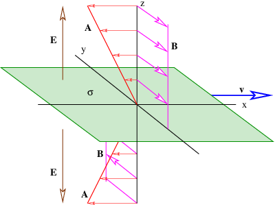
Source: LibreTexts, "Radically Modern Introductory Physics" II
The magnetic potential of a wire
Let us consider the example of the vector potential of a wire segment oriented along the horizontal axis between $x = x_1$ and $x = x_2$ carrying constant current $I$. Since the vector potential is parallel to the current, we only need to calculate the $A_x$ component. If we really wanted to, we could solve Poisson's equation for the magnetic potential $\nabla^2 A_x = -\mu_0 J_x$, but the boundary conditions are non-trivial and it is much easier to use the integral expression instead. Note that $\mathbf{J} = \lambda \hat{\mathbf{x}}$ in this case, where $\lambda$ is the linear charge density of the wire and we integrate over all $dx$. The vector potential is zero for all components except for the $x$-component, since we know that the vector potential always flows parallel to the surface current. The calculation is thus as follows:
$$ \begin{align*} \mathbf{A} &= \dfrac{\mu_0}{4\pi} \int \dfrac{\mathbf{J}(\mathbf{r}')}{| \mathbf{r} - \mathbf{r}'|}dV' \\ \Rightarrow \mathbf{A}_x &= \dfrac{\mu_0}{4\pi} \underbrace{\int_{x_1}^{x_2} \dfrac{\lambda dx'\hat{\mathbf{x}}}{\sqrt{r^2 + x^2}}}_\text{integrate along wire} \end{align*} $$
If we let the bounds of integration be $x_1 = -\infty$ and $x_2 = \infty$ this integral diverges, since the wire is, after all, infinitely long! However, if we choose to let the bounds be finite, then (after looking up an integral table or using Mathematica) we get a "sane" answer, which is given by:
$$ \mathbf{A}_x = \dfrac{\mu_0 I}{4\pi} \hat{\mathbf{x}} \left[\ln(x + \sqrt{r^2 + x^2})\right]_{x_1}^{x_2} $$
This may look ridiculously complicated and make you wonder why anyone would want to use the vector potential, but let us assume that $x_1 = -L$ and $x_2 = L$, where the length of the wire is given by $2L$. This gives:
$$ \mathbf{A} = \mathbf{A}_x = \dfrac{\mu_0 I}{4\pi} \hat{\mathbf{x}} \ln\left[\dfrac{L + \sqrt{r^2+ L^2}}{-L + \sqrt{r^2 + L^2}}\right] \approx \dfrac{\mu_0 I}{4\pi} \hat{\mathbf{x}} \ln \left[\dfrac{4L^2}{r^2}\right], \quad L \gg r $$
Remember that this can also be written as $\mathbf{A} = \dfrac{\mu_0 I}{4\pi}\hat{\mathbf{x}}[\ln(4L^2) - \ln(r^2)]$ via the properties of logs. If we take the curl in cylindrical coordinates, we find that:
$$ \begin{align*} \mathbf{B} &= \nabla \times \mathbf{A} \\ &= \cancel{\left({\frac {1}{r}}{\frac {\partial \mathbf{A}_{x}}{\partial \phi }}-{\frac {\partial \mathbf{A}_{\phi }}{\partial x}}\right){\hat {\mathbf {r }}}} +\left(\cancel{{\frac {\partial \mathbf{A}_{r }}{\partial x}}}-{\frac {\partial \mathbf{A}_{x}}{\partial r }}\right){\hat {\boldsymbol {\phi }}} +\cancel{{\frac {1}{r }}\left({\frac {\partial (r \mathbf{A}_\phi)}{\partial r }}-{\frac {\partial \mathbf{A}_r}{\partial \phi }}\right){\hat {\mathbf {x}}}} \\ &= -\dfrac{\partial \mathbf{A}_x}{\partial r} \hat{\boldsymbol{\phi}} \\ &= -\dfrac{\mu_0I}{4\pi} \hat{\boldsymbol{\phi}} \dfrac{\partial}{\partial r}(\underbrace{\ln(4L^2)}_\text{const.}-\ln(r^2)) \\ &= \dfrac{\mu_0I}{2\pi r}\hat{\boldsymbol{\phi}} \end{align*} $$
This result is simply the magnetic field around a wire of constant current $I$! Thus, we have established that the magnetic potential does indeed produce the same results (and contain essentially the same information) as the magnetic field. It also tells us that the magnetic potential (which points along $\hat{\mathbf{x}}$) and the magnetic field (which points along $\hat{\boldsymbol{\phi}}$) are always pointing perpendicular to each other, as we expected.
The magnetic potential inside a solenoid
We know from earlier that the magnetic field of a solenoid is a constant, and is given by $\mathbf{B} = \mu_0 n I \hat{\mathbf{x}}$. But what is its magnetic potential? Well, if we just use the integral formula for $\mathbf{A}$ we can get the result from brute-force integration. However, there is a more elegant way. note that by Stoke's theorem from vector calculus, we have:
$$ \int \limits_\text{loop} \mathbf{A} \cdot d\mathbf{r} = \int \limits_\text{surface} (\nabla \times \mathbf{A}) \cdot d\mathbf{A} $$
But we know that $\nabla \times \mathbf{A} = \mathbf{B}$, so we have:
$$ \int \limits_\text{surface} (\nabla \times \mathbf{A}) \cdot d\mathbf{A} = \int \limits_\text{surface} \mathbf{B} \cdot d\mathbf{A} = \Phi_B $$
Where $\Phi_B$ is the flux of the magnetic field through the solenoid. Since the magnetic field is given by $\mathbf{B} = \mu_0 n I \hat{\mathbf{x}}$ and flows along $\mathbf{x}$, its flux about a circle of radius $r$ is just:
$$ \Phi_B = \mu_0 n I A = \mu_0 n I \pi r^2 $$
Thus we have:
$$ \int \limits_\text{loop} \mathbf{A} \cdot d\mathbf{r} = \Phi_B = \mu_0 n I \pi r^2 $$
Here we can make two simplifications. First, we know that the magnetic potential always flows in the same direction as the current (well, technically "current" is the surface current, but here there's only one type of current anyways since we assume infinitely-thin wires in the solenoid). This means that the only nonzero component of $\mathbf{A}$ is $\mathbf{A}_\phi$, since the current is flowing along $\phi$ (circularly). Additionally, the line integral of $\mathbf{A}$ around our chosen circle is just multiplying $\mathbf{A}_\phi$ by its circumference, i.e. $2\pi r |\mathbf{A}_\phi|$. Thus, we have:
$$ \int \limits_\text{loop} \mathbf{A} \cdot d\mathbf{r} = 2\pi r |\mathbf{A}_\phi| = \mu_0 nI \pi r^2 $$
Our result is thus:
$$ \mathbf{A}_\phi = \dfrac{\mu_0n I\pi r^2}{2\pi r} = \dfrac{\mu_0n I}{2}r \hat{\boldsymbol{\phi}} $$
This result is linear in $r$, which makes sense, because the derivative of a linear function is simply a constant, and we know that the magnetic field $\mathbf{B} = \mu_0 n I \hat{\mathbf{x}}$ is constant.
The magnetic potential inside a toroid
We now consider a toroidal solenoid (also called a toroid), a variation of the standard solenoid, which is shown in the figure below:

Source: HyperPhysics
Toroids find numerous applications, particularly in nuclear fusion reactors and particle accelerators, so this is indeed an important case to analyze. The magnetic field inside a toroidal solenoid is $\mathbf{B}_\text{toroid} = \dfrac{\mu_0 NI}{2\pi r}\hat{\boldsymbol{\phi}}$, which we can get from Ampere's law. We know that the magnetic vector potential must be perpendicular to the magnetic field and along the direction of the current (which loops up and down in square loops), so we know that it must be along the $z$ axis and thus $\mathbf{A} = \mathbf{A}_z(r)$. Since a toroid is symmetric along $z$ and $\phi$, we know that $\mathbf{A}_z$ is solely dependent on $r$.
Unfortunately, in this case, we cannot use the method we used for the simple (linear) solenoid, since the line integral of $\mathbf{A}$ along the boundary of any surface would depend on $r$. Instead, we can use the definition of $\mathbf{A}$:
$$ \begin{align*} \mathbf{B} &= \nabla \times \mathbf{A} \\ &= \cancel{\left({\frac {1}{r}}{\frac {\partial \mathbf{A}_{z}}{\partial \phi }}-{\frac {\partial \mathbf{A}_{\phi }}{\partial z}}\right){\hat {\mathbf {r }}}} +\left(\cancel{{\frac {\partial \mathbf{A}_{r }}{\partial z}}}-{\frac {\partial \mathbf{A}_{z}}{\partial r }}\right){\hat {\boldsymbol {\phi }}}+\cancel{{\frac {1}{r }}\left({\frac {\partial (r \mathbf{A}_\phi)}{\partial r }}-{\frac {\partial \mathbf{A}_r}{\partial \phi }}\right){\hat {\mathbf {z}}}} \\ &= -\dfrac{\partial \mathbf{A}_z}{\partial r} \hat{\boldsymbol{\phi}} \end{align*} $$
Now equating with our known expression for the field, we have:
$$ -\dfrac{\partial \mathbf{A}_z}{\partial r}\hat{\boldsymbol{\phi}} = \dfrac{\mu_0 NI}{2\pi r}\hat{\boldsymbol{\phi}} $$
We can simply integrate both sides to give us:
$$ \mathbf{A}_z = -\dfrac{\mu_0 NI\hat{\mathbf{z}}}{2\pi} \ln(r) + \text{constants} $$
This result is only valid inside the toroid itself, however. The full solution that is valid both inside and outside the toroid is plotted below:

Source: Wikipedia
The magnetic potential of a perfect magnetic dipole
Let us now consider one of the most (if not the most) important magnetic potentials out there: the magnetic potential for a circular loop of radius $R$ placed on the $xy$ plane. The exact expression for the magnetic potential is very, very complicated. In fact, it is so complicated we will not even write it here. But if we shrink the loop, we find that we get the magnetic field of a perfect magnetic dipole in the limiting case as the loop grows infinitely small:
$$ \begin{matrix*} \mathbf{A} = \dfrac{\mu_0}{4\pi} \dfrac{\mathbf{m} \times \hat r}{r^2} = \dfrac{\mu_0}{4\pi} \dfrac{\mathbf{m} \times \mathbf{r}}{r^3}, &\mathbf{m} = I \cdot A \hat{\mathbf{k}} \end{matrix*} $$
Notice how the magnetic moment $\mathbf{m} = I \cdot A\hat{\mathbf{k}}$ is that of a tiny circular loop of current of radius $R$ that has area $A = \pi R^2$. And we can of course find the magnetic field produced by such a dipole with the familiar formula:
$$ \mathbf{B} = \nabla \times \mathbf{A} = \nabla \times \dfrac{\mu_0}{4\pi}\left(\dfrac{\mathbf{m} \times \mathbf{r}}{r^3}\right) $$
This is one of the few (classical) cases in which the magnetic potential is more fundamental than the magnetic field, and where it is easier to derive the magnetic potential than the magnetic field. Indeed, the dipole is a fundamental model for everything from planetary magnetic fields to the tiny magnetic fields of subatomic particles! A few common formulas for the magnetic moment are shown as follows:
| Physical situation | Expression for $\mathbf{m}$ |
|---|---|
| Loop of current with cross-sectional area $A$ | $\mathbf{m} = (\boldsymbol{I} \cdot A)\hat{\mathbf{k}}$ |
| Charged particle undergoing rotational motion with angular momentum $\mathbf{L}$ | $\mathbf{m} = \gamma \mathbf{L}$ where $\gamma$ is called the gyromagnetic ratio |
| Solenoid along $x$ axis with cross-section $S$ | $\mathbf{m} = NIS \hat{\mathbf{x}}$ |
Additional information: Magnetic dipoles can be divided between two primary types. The first type are physical magnetic dipoles (magnets with two poles and nonzero size, like bar magnets). The second type are ideal magnetic dipoles (which is the limiting case of both an infinitesimally-tiny loop of current and of a physical dipole shrunk infinitely small). While both can be modelled with the same magnetic potential as a perfect dipole, only physical dipoles can exist in real life.
The multipole expansion of the vector potential
Just like the multipole expansion for the electric potential, a similar multipole expansion can be written for the magnetic vector potential (as long as we only consider magnetostatics). The multipole expansion for $\mathbf{A}$ is given by:
$$ \begin{align*} \mathbf{A}(\mathbf{r}) &= \dfrac{\mu_0 I}{4\pi} \sum_{l = 0}^\infty \dfrac{1}{r^{l + 1}} \oint {r'}^l P_l(\cos \theta) dl' \\ &= \dfrac{\mu_0 I}{4\pi} \left[0 + \dfrac{\mathbf{m} \times \mathbf{r}}{r^3}+ \dots\right] \end{align*} $$
Where $P_\ell(x)$ are the Legendre polynomials that we mentioned earlier, and the integration is performed along a closed path with line element $dl'$. Notice how the first term in the multipole expansion for $\mathbf{A}$ is actually zero. This is equivalent to the statement that there are no magnetic monopoles, or essentially, there can be no isolated north or south magnetic pole! Meanwhile, if we take our loop to be a circular loop, the second term is the same result as a perfect magnetic dipole!
A proof of Gauss's law for magnetism from the magnetic potential
We will end with a short and incredibly beautiful proof of Gauss's law for the magnetic field. Recall that the magnetic potential is defined by $\mathbf{B} = \nabla \times \mathbf{A}$. We know that Gauss's law for the electric field is given by $\nabla \cdot \mathbf{E} = \rho/\varepsilon_0$. But if we try to write a similar equation with $\mathbf{B}$, we find that:
$$ \nabla \cdot \mathbf{B} = \nabla \cdot (\nabla \times \mathbf{A}) = 0 $$
Which comes from the vector calculus identity that the divergence of the curl is always zero, that is, $\nabla \cdot (\nabla \times \mathbf{F}) = 0$ for any function $\mathbf{F}$. Thus we have just derived Gauss's law for magnetic fields, $\nabla \cdot \mathbf{B} = 0$! And of course, we can use the divergence theorem to be able to put the differential form of Gauss's law for magnetic fields into integral form:
$$ \int \nabla \cdot \mathbf{B} \, dV = 0 \Rightarrow \oint \mathbf{B} \cdot d\mathbf{A} = 0 $$
Which is exactly the integral form of Gauss's law for magnetic fields that we know! Thus, the magnetic potential automatically guarantees that $\nabla \cdot \mathbf{B} = 0$. This is a hint of what we'll see in detail later: the magnetic potential gives us a way of simplifying the four Maxwell equations into just one equation, making it incredibly useful.
Magnetic fields inside matter
Magnetism has a crucial difference as compared to electrostatics: point charges exist in electrostatics, but "point magnets" (also called magnetic monopoles) do not exist. The closest analogue to a point charge in magnetism is the magnetic dipole. Magnetic dipoles are an arrangement of two charges of opposite charge; the two ends are called magnetic poles (or just poles) and generate a characteristic magnetic field. This field has field lines that begin at one pole and end at another pole, as shown in the drawing below:

Source: Wikipedia
The magnetic field of a bar magnet, as well as Earth's planetary magnetic field, are examples of (non-ideal) dipoles. Using the Biot-Savart law, the magnetic field of a magnetic dipole can be found to be:
$$ \mathbf{B}_\text{dipole} = \dfrac{\mu_0}{4\pi} \nabla \times \left(\mathbf{m} \times \dfrac{\hat r}{r^2}\right) = \dfrac{\mu_0}{4\pi} \left(\dfrac{3\hat{\mathbf{r}}(\hat{\mathbf{r}} \cdot \mathbf{m}) - \mathbf{m}}{|\mathbf{r}|^3}\right) $$
Which comes from the magnetic vector potential of a magnetic dipole, given by:
$$ \mathbf{A}_\text{dipole} = \dfrac{\mu_0}{4\pi}\left(\mathbf{m} \times \dfrac{\hat r}{r^2}\right) $$
Where $\mathbf{m}$ is called the magnetic moment, which is similar in some ways (but not identical) to the electric dipole moment. We can show (but we don't derive here) that a perfect dipole has the same magentic field as a tiny loop of current shrunk infinitesimally-tiny, whose magnetic moment is given by the integral over the cross-sectional area of the loop:
$$ \mathbf{m} = I\int d\mathbf{A} $$
The magnetization of a material is given by $\mathbf{M}$, where $N$ is dipole density (dipoles per unit volume, which is generally equivalent to the number of atoms per unit volume):
$$ \mathbf{M} = N(\mathbf{m} \cdot \mathbf{r})_\text{average} $$
Atomic magnetism and magnetic materials
Before we begin this section, we should warn that we discuss quite a bit of quantum mechanics in this section (albeit with relatively little mathematics). Please consult the quantum physics guide if you are not familiar with quantum physics.
When a magnetic dipole is placed in a magnetic field, it experiences a torque that causes the dipole to orient parallel to the field lines, increasing the total strength of the magnetic field. The precise expression for the torque is given by:
$$ \vec \tau = \mathbf{m} \times \mathbf{B} $$
This effect is known as paramagnetism, and while it can be described in classical terms, the full explanation for why it exists comes from quantum mechanics. In quantum mechanics, we find that the origin of magnetic moments comes from the orbital angular momentum of atoms, and spin angular momentum of their electrons. The sum total of these effects leads to a magnetic moment that is given by:
$$ \mathbf{m} = -g \mu_B \mathbf{J} $$
Where $\mathbf{J} = \langle J_x, J_y, J_z \rangle$ are the values of the angular momentum (which, for those familiar with quantum mechanics, are the eigenvalues of the spin-included total angular momentum operator $\hat J$), $g$ is a constant known as the gyromagnetic ratio, and $\mu_B \approx \pu{9.274E-24 J*T^{-1}}$ is a universal constant known as the Bohr magneton. Paramagnetism is usually an extremely weak effect that is barely observable, except at very small scales or in strong magnetic fields.
Another type of weak magnetism, distinct from paramagnetism, is known as diamagnetism. Diamagmentism comes from an effect called electromagnetic induction, which we will cover more on later. Electromagnetic induction comes from the fact that a dipole placed in an external magnetic field induces a magnetic field pointing in the opposite direction. This induced field repels the applied external field, leading to the dipole orienting anti-parallel (parallel but in the opposite direction) to the field lines. Like paramagnetism, it is a very weak effect that is extremely hard to observe.
Ferromagnetism is an extremely rare effect and gives rise to permanent magnets. Only a few materials exhibit ferromagnetism, most notably iron, which is the origin of the name ferromagnetism (the elemental symbol for iron is $\ce{Fe}$). Ferromagnetism arises from quantum-mechanical effects; for those familiar, it comes from a peculiar property of electrons called spin, which can be imagined as a vector that can only point up or down. Electrons can have one of two spins, typically called spin-up and spin-down. When all the electrons have paired spins, their magnetic moments fully align in the same direction, creating very strong magnetic fields (relative to the size of atoms), strong enough to be easily observable macroscopically. Crucially, no external field is required for a material to exhibit ferromagnetism; it is a property of the material itself.
Note for the advanced reader: there are also two related types of magnetism, which are known as ferrimagnetism and anti-ferromagnetism. They also arise without needing an external field, although they come from opposite (instead of paired) spins.
Ferromagnetism alone does not explain permanent magnets - after all, if we naively assume that all ferromagnetic materials have fully-aligned magnetic moments, then every piece of iron should attract each other, including the iron atoms in your blood! This obviously does not happen, and the reason is that while ferromagnetic materials have electrons with paired spins (and thus aligned magnetic moments), regions of ferromagnetic materials may be aligned differently. These regions are called domains, which we show in the image below:
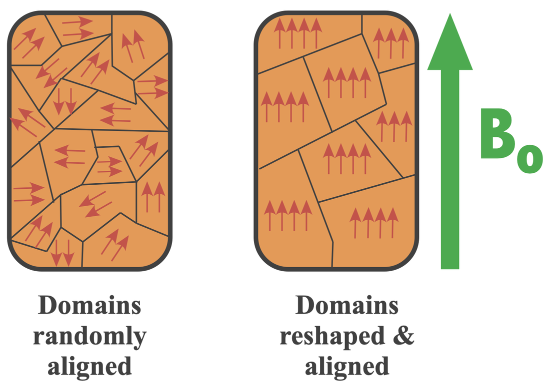
Source: MRI Questions by Elster LLC. Displayed under fair use.
When the domains are randomly-aligned, their magnetic moments cancel out, and no net magnetic field arises. But when an external magnetic field (such as that of a solenoid) is applied, each domain experiences a torque that aligns the domains along the same direction. When the field is removed, the domains are now aligned, and ferromagnetic material is now a permanent magnet.
Note: For a funny, educational video about the origins of magnetism that summarizes atomic magnetism very well, see the Magnets video by MinutePhysics on YouTube.
Magnetization
Just like materials can be electrically polarized, they can also be magnetically polarized, or as it is more commonly called, magnetized. The magnetization field (or more simply, just referred to as the magnetization) of a material, $\mathbf{M}$, is given by the total contribution of the individual magnetic dipole moments in the material, per unit volume:
$$ \mathbf{M} = \dfrac{1}{V} \sum_i \mathbf{m}_i $$
Alternatively, in continuous materials, we have:
$$ \mathbf{M} = \dfrac{d\mathbf{m}}{d V}, \quad \mathbf{m} = \iiint \mathbf{M} ~dV $$
The magnetization is very similar to polarization field ($\mathbf{D}$ field) from electrostatics. In fact, we can characterize the magnetization in terms of a bound current and free current, just like the bound and free charge in electrostatics. Again, just as in electrostatics, the magnetic dipole moments typically cancel out within the material, with two exceptions: the dipoles at the material's surface, and the dipoles within non-uniform regions within the interior of the material. This is just like the surface bound charge and volume (interior) bound charge! Since we can speak of perfect magnetic dipoles as equivalent to tiny current loops, the magnetized material essentially has a current circulating within the interior of the material as well as a current circulating around its surface. We may then define the bound surface current $\mathbf{K}_b$ and the bound volume current $\mathbf{J}_b$ as follows:
$$ \begin{matrix*} \mathbf{K}_b = \mathbf{M} \times \hat{\mathbf{n}}, &\mathbf{J}_b = \nabla \times \mathbf{M} \end{matrix*} $$
Notice how this is in many ways very similar to the equivalents ($\mathbf{D}$ and $\mathbf{P}$) for electric fields in matter! Indeed, we can also separated the magnetic field into a "free" field ($\mathbf{H}$) and a magnetization field ($\mathbf{M}$), and the magnetic field in matter also satisfies a constitutive relation:
$$ \mathbf{B} = \mu_0(\mathbf{H} + \mathbf{M}) $$
Note: For complicated reasons, $\mathbf{H}$ is commonly called the demagnetizing field. However, to avoid confusion, we will continue calling it the $\mathbf{H}$ field.
In addition, the $\mathbf{H}$ field satisfies Ampere's law in matter, which is given by:
$$ \nabla \times \mathbf{H} = \mathbf{J}_f $$
Where $\mathbf{J}_f$ is the free current inside the material, and the total current density $\mathbf{J}$ is given by:
$$ \mathbf{J} = \mathbf{J}_f + \mathbf{J}_b $$
Most everyday materials are magnetically-linear materials and respond very weakly when placed inside magnetic fields. The exception, of course, is with ferromagnetic materials, which (certainly!) do not respond linearly to applied magnetic fields, leading to their spectacular magnetic properties. However, if we simply consider linear materials, we have:
$$ \mathbf{M} = \chi_m \mathbf{H}, \quad \mathbf{B} = \mu_0 (1 + \chi_m) \mathbf{H} = \mu \mathbf{H} $$
where $\chi_m$ is the magnetic susceptibility and $\mu = \mu_0(1 + \chi_m)$ is the material permeability.
Note: For more resources on magnetic materials and magnetization, see this study guide and these lecture guides by the University of Texas.
Electromagnetic induction
Up to this point, we have discussed static electric fields and magnetic fields, which come from slow-moving charges (for electrostatic fields) and constant currents (for magnetic fields). But now is the time for us to examine when the static assumptions no longer hold. This is the domain of electrodynamics.
The Lorentz force and motional EMF
Consider a conductor immersed in some uniform magnetic field $\mathbf{B}$ that moves at velocity $\mathbf{v}$. For instance, this could be a metal rod sliding on a railing. Let us consider an unusual question: what is the potential difference caused by the Lorentz force acting on the rod? Well, we know that potential difference is formally defined as:
$$ V = -\int_a^b \mathbf{E} \cdot d\mathbf{r} = -\dfrac{1}{q} \int_a^b \mathbf{F}_E \cdot d\mathbf{r} $$
Where $\mathbf{F}_E = q\mathbf{E}$ is the electric force. This definition tells us that the potential difference between two locations is equivalent to the energy put in to move a charge $q$ between the two locations, against the electric field. But what if we generalize this to the Lorentz force $\mathbf{F}_{EM} = q\mathbf{E} + q\mathbf{v} \times \mathbf{B}$? The answer is now not as simple as it seems. The Lorentz force is non-conservative, so its line integral around a closed loop is nonzero. Thus, we have:
$$ \begin{align*} V &= \dfrac{1}{q}\oint_C \mathbf{F}_{EM} \cdot d\mathbf{r} \\ &= \dfrac{1}{q} \oint_C q(\mathbf{E} + \mathbf{v} \times \mathbf{B}) \cdot d\mathbf{r} \\ &= \oint_C (\mathbf{E} + \mathbf{v} \times \mathbf{B}) \cdot d\mathbf{r} \end{align*} $$
We see that the potential difference is now a very strange sort of potential difference, which comes from both the electric and magnetic fields acting on the conductor. While there was no electric field to begin with, the movement of the conductor through the magnetic field ends up generating a Lorentz force that pushes charges through a potential difference, causing them to create an electric field!
In fact, we usually represent this "pseudo-potential-difference" with the symbol $\mathcal{E}$ rather than $V$, since it is not the result of any pre-existing electric field, but rather a result of the motion of a conductor through an ambient magnetic field. The symbol $\mathcal{E}$ comes from the (misleading) historical name of this potential difference of "electromotive force" (EMF for short). More formally, we call it the motional EMF, since we observe it only when $\mathbf{v} > 0$, when the conductor is moving through the magnetic field!
Faraday's law and electromagnetic induction
Similar to the electric flux, we define the magnetic flux $\Phi_B$ as the surface integral of the magnetic field across some given surface:
$$ \Phi_B = \iint \mathbf{B} \cdot d\mathbf{A} $$
Note: Be careful that the surface in question is not a Gaussian surface, since it is not closed. By Gauss's law for the magnetic field, the magnetic flux through a Gaussian surface is always zero!
Let us now consider a wire loop that is immersed in some magnetic field $\mathbf{B}$ whose total magnetic flux through the loop varies with time. Unlike motional EMF, which we have previously discussed, our wire loop is not necessarily moving; it is only the flux through the loop is changing. In fact, there are three cases which can cause changing flux through the loop:
- The wire loop is moving in a non-uniform magnetic field, that is, $\mathbf{B} = \mathbf{B}(\mathbf{r})$ has spatial dependence
- The wire loop is not moving, but rotates in place through a uniform magnetic field $\mathbf{B} = \mathbf{B}_0$
- The wire loop is stationary, but the magnetic field is time-dependent, that is, $\mathbf{B} = \mathbf{B}(t)$
We show each of these cases below. In case (1), we have a magnetic field that depends on position - it is equal to $\mathbf{B} = \mathbf{B}_0$ for $x \leq a$ and $\mathbf{B} = 0$ for $x > a$. In case (2), we have a loop that is rotating within a magnetic field; since the flux $\Phi = \mathbf{B}\cdot \mathbf{A} = |B||A|\cos \theta$ depends on the angle between the loop and the magnetic field vectors, there is a change in flux as the loop rotates, and therefore an EMF. Lastly, in case (3), we have a time-dependent magnetic field, so the flux through the loop is also changes with time.

Reference: MITx electromagnetic theory
We can go through even more examples. For instance, consider a bar magnet that moves through a loop. The loop itself is not moving, but since the magnet is moving, the magnetic flux through the loop changes. Or conside a loop that slowly moves away from a wire. Remember, the magnetic field around a long wire is given by $\mathbf{B}(\mathbf{r}) = \dfrac{\mu_0 I}{2\pi r} \hat r$ - so, if we have a loop moving in the $r$ direction away from the wire, the flux changes (decreases) over time.

Faraday found experimentally that in all three cases, the changing magnetic flux through the loop (not the flux itself, the rate of change of the flux) actually produces an EMF. We call this type of EMF as the induced EMF (though we can get sloppy and call it just "the EMF" sometimes). The induced EMF is given by:
$$ \mathcal{E} = \oint \mathbf{E} \cdot d\mathbf{r} = -\dfrac{d}{dt} \iint \mathbf{B} \cdot d\mathbf{A} $$
Note: be careful that by "flux" in Faraday's law, we always mean total flux (which is also called the flux linkage). This is especially relevant for the flux of a magnetic field through a solenoid, which is composed of a large number of loops. The individual flux through one loop might be small, but the total flux through all of the loops can be very large!
We can use Stoke's theorem from vector calculus ($\displaystyle \oint \mathbf{E} \cdot d\mathbf{r} = \displaystyle \iint \nabla \times \mathbf{E}\cdot d\mathbf{A}$) to rewrite Faraday's law in its differential form:
$$ \nabla \times \mathbf{E} = -\dfrac{\partial \mathbf{B}}{\partial t} $$
From which we can more clearly see that a magnetic field changing over time is bound to produce an induced circulating electric field. This induced electric field has some very special characteristics:
- It is a non-conservative field
- It has closed field lines, just like a magnetic field, and
- It can exist in free space, even far away from any charges!
Interestingly, Faraday's law is the exact same equation whether you derive it through motional EMF due to the Lorentz force or the induced EMF coming from an induced electric field due to a time-varying magnetic field. This is a very deep insight that led Einstein to develop his special theory of relativity!
Addenum: the potential formulation from Faraday's law
Remember that we said that the induced electric field $\mathbf{E}$ is non-conservative, so it would appear that the electrostatic potential $V$ (which is conservative) is of no use to describe induced electric fields. But there is a way to describe an induced field in terms of potentials. Remember that we have defined the magnetic vector potential as $\mathbf{B} = \nabla \times \mathbf{A}$. Since the magnetic field is non-conservative anyways, this relation still holds true in the case of electromagnetic induction. If we substitute this into the differential form of Faraday's law, we have:
$$ \nabla \times \mathbf{E} = -\dfrac{\partial \mathbf{B}}{\partial t} = -\dfrac{\partial}{\partial t} (\nabla \times \mathbf{A}) = \nabla \times \left(-\dfrac{\partial \mathbf{A}}{\partial t}\right) $$
(Here we can switch around the time derivative and the curl by a vector calculus identity). But this equation is not precisely correct, because if we add the gradient of an arbitrary function, since the curl of a gradient is zero, the equation would still hold true:
$$ \begin{align*} -\dfrac{\partial}{\partial t} (\nabla \times \mathbf{A} + \nabla f) &= \nabla \times \left(-\dfrac{\partial \mathbf{A}}{\partial t} + \nabla f\right) \\ &=\nabla \times \left(-\dfrac{\partial \mathbf{A}}{\partial t}\right) + \cancel{\nabla \times \nabla f} \\ &= \nabla \times \left(-\dfrac{\partial \mathbf{A}}{\partial t}\right) \end{align*} $$
This suggests that if we let $\nabla f = -\nabla V$, the electric potential, then we can rewrite Faraday's law as:
$$ \nabla \times \mathbf{E} = \nabla \times \left(-\dfrac{\partial \mathbf{A}}{\partial t} - \nabla V\right) $$
From which we may define the electric field purely in terms of potentials as:
$$ \mathbf{E} = -\nabla V - \dfrac{\partial \mathbf{A}}{\partial t} $$
This is the preferred formulation in relativistic quantum mechanics, particle physics, and advanced theoretical physics in general, although we will not go too in-depth within this guide.
Inductance and inductors
In Faraday's law, we find that interestingly, there is a negative sign on the right-hand side. That is, a faster change in flux results in a smaller EMF, while a slower change in flux results in a larger EMF. It is almost as if there is some "invisible" force that is opposing the change in flux!
Indeed, this is a real effect, called Lenz's law. And it does not come from an invisible force - we find that an induced electric field produced by a changing magnetic flux itself creates a magnetic field that opposes the change in flux. This means that as the magnetic flux changes, which induces an EMF that (in a conducting loop) drives a current through a loop, that current itself induces an opposing magnetic field which tries to push against that current by inducing a magnetic field in the opposite direction. This opposing magnetic field tries to "drive down" the current from the EMF, which produces a change in current $\dfrac{dI}{dt}$. We illustrate this situation below:

The rate of change of the this current is proportional to the change in flux, and we call this proportionality constant the inductance, symbol $L$. Thus, Lenz's law is given by:
$$ \mathcal{E} = -\dfrac{d\Phi_B}{dt} = -|L| \dfrac{dI}{dt} $$
Since the EMF generates an opposing magnetic field, it can be thought of as "pushing back" against the original magnetic field and opposing the change in current. Thus, we say that $\mathcal{E}$ is a special type of EMF, called back EMF, and the equation for finding the back EMF is Lenz's law. If we integrate both sides, we can find an explicit expression for $L$, as shown:
$$ \begin{align*} \int-\dfrac{d\Phi_B}{dt} &= \int-|L| \dfrac{dI}{dt} \\ \Phi_B &= L I \\ \Rightarrow L = \dfrac{\Phi_B}{I} \end{align*} $$
But if this effect occurs, how is it possible that the change in current doesn't exactly cancel out the induced EMF? The answer is that in most cases, $L$ is very small, so the induced EMF dominates. There are, however, ways to greatly increase where $L$ can be made quite large, which is very important for devices called inductors - which we'll look at next!
Self-inductance
When inductance occurs in the same loop (or coil) as the loop (or coil) where the magnetic field produces an EMF, we call this type of inductance self-inductance. Usually, this type of inductance is unwanted, because it decreases the induced current through the coil/loop; in most applications, we want the induced current to be as high as possible, so we say that the self-inductance is parasitic. However, there are some applications where self-inductance is desired: for instance, electrical devices are often shielded with inductors, devices that have a high inductance, to prevent rapid changes in current (such as power surges) from destroying the device. In this part, we will calculate the inductance of a few simple inductors.
To start things off, we will consider a relatively straightforward example. Consider a solenoid formed by $N$ circular loops of radius $R$, with a total length of $L$ and $n = N/L$ turns per unit length. We show this in the diagram below:

The solenoid has a current $I(t)$ that passes through it, which produces a time-varying magnetic field $\mathbf{B}(t) = \mu_0 n I(t) \hat x$, causing a changing flux. We can calculate the magnetic flux across a single pool as follows:
$$ \Phi_B = \iint \mathbf{B} \cdot d\mathbf{A} = \mathbf{B} \cdot \mathbf{A} = \mu_0 n I(t) \pi R^2 $$
But given that there are $N$ turns in the solenoid, the total flux would be:
$$ \Phi_T = N \Phi_B =\mu_0 nN I(t) \pi R^2 = \dfrac{\mu_0 \pi R^2N^2}{L}I(t) $$
The self-inductance would simply be the total flux divided by the current, so we would have:
$$ L = \dfrac{\Phi_T}{I} = \dfrac{\mu_0 \pi R^2N^2}{L} $$
Notice that the self-inductance is a constant that doesn't depend on the current or time, and only depends on the geometric qualities of the solenoid. This is very similar to capacitance, which also depends only on the geometric qualities of a capacitor. We will see this parallel come up again later.
Let us consider a more challenging example: calculating the self-inductance of a toroidal solenoid (toroid) of radius inner radius $a$, outer radius $b$, and height $h$ with $N$ turns. A toroid looks very similar to a standard solenoid, but with the ends joined together, as is shown in the diagram below:
Source: HyperPhysics
By Ampere's law we find the field of a toroid to be:
$$ \mathbf{B} = \dfrac{\mu_0 NI}{2\pi r} \hat \theta $$
This means that the flux in one turn of the toroid would be given by:
$$ \Phi_B = \iint \mathbf{B} \cdot d\mathbf{A} = \int_0^h \int_a^b \dfrac{\mu_0 NI}{2\pi r} dr dz = \dfrac{\mu_0 h}{2\pi} N I \ln\left(\dfrac{b}{a}\right) $$
This is just one turn, but we know the toroid has $N$ turns, so the total flux would be:
$$ \Phi_T = N \Phi_B = \dfrac{\mu_0 h}{2\pi} N^2 I \ln\left(\dfrac{b}{a}\right) $$
And thus the self-inductance becomes:
$$ L = \dfrac{\Phi_T}{I} = \dfrac{\mu_0 h}{2\pi} N^2 \ln\left(\dfrac{b}{a}\right) $$
Mutual inductance
So far, we have seen the case of electromagnetic induction around one loop (or at least, one coil) of wire. But there is no reason why we can't generalize this to two loops (or coils)! If we choose to put another coil after the first coil (we will say "loop" and "coil" interchangeably here), we may readily calculate the total flux from the first coil $\Phi_\text{from 1}$ passing through the second coil as follows:
$$ \Phi_\text{from 1} = \iint \limits_\text{coil 2} \mathbf{B}_1 \cdot d\mathbf{A} $$
The total flux $\Phi_\text{from 1}$ caused by the magnetic field from the first coil passing through the second coil creates an EMF (and therefore drives a current) in the second coil, which is opposed by the induced magnetic field due to the current (by Lenz's law). We show this in the drawing below:

We call this effect mutual inductance, denoted $M$, and is given by:
$$ M = \dfrac{\Phi_\text{from 1}}{I_2} $$
That is, the mutual inductance is the ratio between $\Phi_\text{from 1}$, the magnetic field from the first loop/coil, to $I_2$, the current in the second loop/coil. We may arbitrarily choose which loop/coil we call "coil 1" and which coil we call "coil 2", because of the mutual inductance theorem. This says that mutual inductance between two loops/coils (or really any two EMF sources) is symmetric, meaning it is independent of your choice of numbering the coils/loops:
$$ M_{ij} = M_{ji} $$
This is very convenient, because in cases where the flux of the magnetic field coming from one coil/loop passing through the other is hard to calculate, it is often much easier to calculate the flux of the magnetic field coming from the other loop.
Mutual inductance is not simply a physical effect; it has important applications, too. For instance, it is the working principle of transformers, which are devices that increase (or reduce) the voltage without dissipating it like a resistor (which wastes energy). Transformers work by using two sets of coils. Time-varying current (usually sinusoidal current in the form $I(t) = I_0 \cos \omega t$) is passed through the first coil, producing a time-dependent magnetic field $\mathbf{B}_1(t)$. The flux of this magnetic field changes with time, which produces an EMF by Faraday's law; the EMF drives a current which is opposed by the induced magnetic field that comes from that current. This decreases the EMF, and therefore the current passing through the second coil, which can be connected to another wire to send current elsewhere. This process can also be used to boost the EMF by using different numbers of windings on the first and second coils. It allows, for instance, current from power stations to be sent to faraway locations by increasing the voltage, where the voltage is then dropped for household use.
Maxwell's equations and electrodynamics
Up to this point, we have collectively seen the four Maxwell's equations in their static form:
$$ \begin{align*} \oint \mathbf{E} \cdot d\mathbf{A} &= Q_\text{enc.}/\varepsilon_0 \\ \oint \mathbf{B} \cdot d\mathbf{A} &= 0 \\ \oint \mathbf{E} \cdot d\mathbf{r} &= -\dfrac{d\Phi_B}{dt} \\ \oint \mathbf{B} \cdot d\mathbf{r} &= \mu_0 I_\text{enc.} \end{align*} $$
In the four equations above, the top three equations are all correct: Gauss's law for electricity, Gauss's law for magnetism, and Faraday's law. But the fourth equation - Ampere's law - is not correct, or at least, not completely correct. It holds true for statics (that is, when electrostatics or magnetostatics applies), but not electrodynamics.
To see why, consider a capacitor on the $+x$ axis, made of two conducting plates some distance $d$ apart, separated by empty space - if you a review of capacitors, see the introductory electromagnetism guide. A current $I$ flows via a wire into one side of the capacitor, charging up one plate. Here is a sketch below:

Source: Physics StackExchange
We have already calculated the electric field of a capacitor (between its two plates) in the introductory electromagnetism guide - it is given by $\mathbf{E} = \dfrac{\sigma}{\varepsilon_0} \hat{\mathbf{x}}$. But what about the magnetic field of a capacitor? You may be inclined to say that there is no magnetic field in the middle of the capacitor; after all, there is no wire there, just the empty space separating the two plates.
But recall that the capacitance of a capacitor is related to its charge by $Q = CV$, so if we take the time derivative of both sides (remember $I = dQ/dt$) and rearrange, we get $I_\text{cap.} = C \dfrac{dV}{dt}$. As the capacitor is charged (or discharged), the potential difference between the plates certainly does change, so there is absolutely current within the capacitor!
So we face a dilemna: there are no actual charges flowing between the capacitor's two plates, but there is current. Ampere's law, at least in the form we have seen it as, does not explain this. But we can modify Ampere's law to account for this "invisible current". Taking inspiration from Faraday's law $\displaystyle \oint \mathbf{B} \cdot d\mathbf{r} = \mathcal{E} = -\dfrac{d\Phi_B}{dt}$, we can include a term that is proportional to the time derivative of the electric field:
$$ \begin{gather*} \oint \mathbf{B} \cdot d\mathbf{r} = \mu_0 \bigg(I_\text{enc.} + \underbrace{\varepsilon_0 \dfrac{d\Phi_E}{dt}}_\text{"current"}\bigg) \\ \Rightarrow \oint \mathbf{B} \cdot d\mathbf{r} = \mu_0 (I_\text{enc.} + I_D), \quad I_D \equiv \varepsilon_0 \dfrac{d\Phi_E}{dt} \end{gather*} $$
This current is called displacement current, denoted $I_D$, is very unusual, because (as we saw) it is not formed by actual moving charge. So we now have two current terms on the right-hand side of Ampere's law: $I_\text{enc.}$ (also called the conduction current) which is the real current formed by moving charges, and $I_D = \varepsilon_0 \dfrac{d\Phi_E}{dt}$ (also called the displacement current), which is the effective current that isn't formed by any actual charge. But just as a changing magnetic flux leads to an induced EMF, Maxwell hypothesized that a changing electric flux leads to an induced displacement current. So if we switch to the differential form of Maxwell's equations and add the displacement current (density) term, we have:
$$ \begin{gather*} \nabla \times \mathbf{B} = \mu_0 (\mathbf{J}_\text{enc.} + \mathbf{J}_D), \quad \mathbf{J}_D = \varepsilon_0 \dfrac{\partial \mathbf{E}}{\partial t} = \dfrac{\partial \mathbf{D}}{\partial t} \\ \Rightarrow \nabla \times \mathbf{B}= \mu_0 \mathbf{J}_\text{enc.} + \mu_0 \varepsilon_0 \dfrac{\partial \mathbf{E}}{\partial t}\quad \text{(Maxwell-Ampere law)} \end{gather*} $$
Ampere's law, modified by Maxwell, is often called the Maxwell-Ampere law. It completes Maxwell's equations, and gives us the modern form of Maxwell that is correct is all situations. Notice that if the electric field does not change, then $\dfrac{d\Phi_E}{dt} = 0$ and thus we recover the "old version" of Ampere's law, $\displaystyle \oint \mathbf{B} \cdot d\mathbf{r} = \mu_0 I_\text{enc.}$.
Note: The term "displacement current" is a terrible name, because it is not really a current in the sense that it does not necessarily consist of any actual moving charges, just like "electromotive force" (also terribly-named) is not a force. Also note that the word "displacement" in "displacement current" refers to the fact that it has units of the $\mathbf{D}$ field over time. Don't take the names too seriously - the mathematics are the better way to gain a physical intuition.
Maxwell's equations in matter with displacement current
In matter, Maxwell's equations must also be modified to take the displacement current into account. The correct form of Maxwell's equations are then given by:
$$ \begin{align*} \nabla \cdot \mathbf{D} &= \rho_f \\ \nabla \cdot \mathbf{B} &= 0 \\ \nabla \times \mathbf{E} &= -\dfrac{\partial \mathbf{B}}{\partial t} \\ \nabla \times \mathbf{H} &= \mathbf{J}_f + \dfrac{\partial \mathbf{D}}{\partial t} \\ \mathbf{D} =& \, \varepsilon_0 \mathbf{E} + \mathbf{P}, \\ \mathbf{H} =& \, \dfrac{1}{\mu_0} \mathbf{B} - \mathbf{M} \end{align*} $$
Where, to incorporate Maxwell's correction to Ampere's law, we must modify our definition of the bound current (density) from $\mathbf{J}_b = \nabla \times \mathbf{M}$ to $\mathbf{J}_b = \nabla \times \mathbf{M} + \dfrac{\partial \mathbf{P}}{\partial t}$, and add a displacement current term $\mathbf{J}_D = \varepsilon_0 \dfrac{\partial \mathbf{E}}{\partial t}$ to Ampere's law. In general, it is not possible to find the (total) electric field $\mathbf{E}$ and magnetic field $\mathbf{B}$ without knowing the exact expressions for $\mathbf{P}$ and $\mathbf{M}$, unless the material is linear, where:
- If we have an electrically-linear material, then $\mathbf{P} = \varepsilon_0 \chi_e \mathbf{B}$, and $\mathbf{D} = \varepsilon \mathbf{E}$ (where $\varepsilon = \varepsilon_0(1 + \chi_e)$), so it is possible to directly solve for the electric field just by finding $\mathbf{D}$.
- Similarly, if we have a magnetically-linear material, then $\mathbf{M} = \chi_m \mathbf{H}$, and so $\mathbf{H} = \mathbf{B}/\mu$ (where $\mu = \mu_0(1 + \chi_m)$), so it is also possible to directly solve for the magnetic field just by finding $\mathbf{H}$.
Note: We have been sloppy with calling materials "linear" without distinguishing between electrically-linear and magnetically-linear materials. A material being electrically-linear does not necessarily mean that the same material is magnetically-linear. Thankfully, most materials are both electrically-linear and magnetically-linear, so we don't have to worry about the distinction. There are, however, some exceptions, such as materials placed under extreme electric fields (where they become electrically non-linear) and (in more everyday conditions) ferromagnetic and antiferromagnetic materials (which are naturally magnetically non-linear).
The theoretical discovery of electromagnetic waves
Let us now consider Maxwell's equations in a very special case: where the charge density and current density are both zero. Then, Maxwell's equations reduce to the much simpler form:
$$ \begin{align*} \nabla \cdot \mathbf{E} &= 0 \\ \nabla \cdot \mathbf{B} &= 0 \\ \nabla \times \mathbf{E} &= -\dfrac{\partial \mathbf{B}}{\partial t} \\ \nabla \times \mathbf{B} &= \mu_0 \varepsilon_0\dfrac{\partial \mathbf{E}}{\partial t} \end{align*} $$
Now, consider the (admittedly-unorthrodox) procedure of taking the curl of Faraday's law. We then have:
$$ \begin{align*} \nabla \times \left(\nabla \times \mathbf{E}\right) &= \nabla \times \left(-\dfrac{\partial \mathbf{B}}{\partial t}\right) \\ &= -\dfrac{\partial}{\partial t} \underbrace{\left(\nabla \times \mathbf{B}\right)}_\text{Ampere's law} \\ &= -\dfrac{\partial}{\partial t}\left(\mu_0 \varepsilon_0\dfrac{\partial \mathbf{E}}{\partial t}\right) \\ &= -\mu_0 \varepsilon_0 \dfrac{\partial^2 \mathbf{E}}{\partial t^2} \end{align*} $$
But note that by the vector calculus identity $\nabla \times (\nabla \times \mathbf{F}) = \nabla(\nabla \cdot \mathbf{F}) - \nabla^2 \mathbf{F}$, we have:
$$ \begin{align*} \nabla \times (\nabla \times \mathbf{F}) &= \nabla(\nabla \cdot \mathbf{F}) - \nabla^2 \mathbf{F} \\ &= \nabla \underbrace{(\nabla \cdot \mathbf{E})}_{\nabla\ \cdot\ \mathbf{E}\ =\ 0} - \nabla^2 \mathbf{E} \\ &= - \nabla^2 \mathbf{E} \end{align*} $$
So putting our two results together, we have:
$$ \begin{gather*} - \nabla^2 \mathbf{E} = -\mu_0 \varepsilon_0 \dfrac{\partial^2 \mathbf{E}}{\partial t^2} \\ \Rightarrow \dfrac{\partial^2 \mathbf{E}}{\partial t^2} = \dfrac{1}{\mu_0 \varepsilon_0} \nabla^2 \mathbf{E} \end{gather*} $$
This is the electromagnetic wave equation (EM wave equation for short), because if we compare it against the standard form of the wave equation $\frac{\partial^2 f}{\partial t^2} = v^2 \nabla^2 f$ (which describes a wave $f(x, t)$ propagating at velocity $v$), we have an exact match if we make the identification $v^2 = 1/\mu_0 \varepsilon_0$. Furthermore, if we solve for $v$, we have:
$$ v = \dfrac{1}{\sqrt{\mu_0 \varepsilon_0}} = \text{299,792,458 m/s} $$
This is exactly the speed of light, $c$! Therefore, by purely invoking the equations of electromagnetic theory, Maxwell was able to predict the existence of electromagnetic waves, and furthermore, show that light is an electromagnetic wave. Thus the EM wave equation is more commonly written as:
$$ \dfrac{\partial^2 \mathbf{E}}{\partial t^2} = c^2 \nabla^2 \mathbf{E} $$
Note that by performing the same mathematical analysis, only starting by taking the curl of Ampere's law ($\nabla \times \nabla \times \mathbf{B}$), we can also arrive at an EM wave equation for the magnetic field:
$$ \dfrac{\partial^2 \mathbf{B}}{\partial t^2} = c^2 \nabla^2 \mathbf{B} $$
The combined vector-valued EM wave equations can be expanded in component form as:
$$ \begin{align*} \dfrac{\partial^2 E_x}{\partial t^2} = c^2 \nabla^2 E_x,& &\dfrac{\partial^2 B_x}{\partial t^2} = c^2 \nabla^2 B_x \\ \dfrac{\partial^2 E_y}{\partial t^2} = c^2 \nabla^2 E_y,& &\dfrac{\partial^2 B_y}{\partial t^2} = c^2 \nabla^2 B_y \\ \dfrac{\partial^2 E_z}{\partial t^2} = c^2 \nabla^2 E_z,& &\dfrac{\partial^2 B_z}{\partial t^2} = c^2 \nabla^2 B_z \end{align*} $$
Maxwell predicted that even far away from sources, electric and magnetic fields in free space can self-propagate, carrying energy and signals over long distances. It is by this principle that the Sun's light is able to heat the Earth and keeps it warm, making life on Earth possible, and by which wireless transmitters producing electromagnetic waves allowed for the invention of modern internet.
Note: It is important to recognize that pure electromagnetic waves are technically only possible in free space, far from sources and charges. We will later discuss the case of what happens when electromagnetic waves interact with matter.
Solutions to the EM wave equation are extremely important, and for good reason. Thankfully, the EM wave equation is separable, so we can use similar methods as we used for solving Laplace's equation to obtain solutions to this partial differential equation. Solutions can be found in Cartesian coordinates, known as plane waves, or in spherical coordinates, yielding spherical waves. More exotic solutions can also be found, such as Gaussian beams, transverse-mode standing waves , and dipole radiation, among others, with specialist applications. These solutions are privotal to radio astronomy, modern telecommunications technology, GPS, the internet, and so, so much more.
Traveling plane-wave solutions to the EM wave equation
We will first consider the simplest solution to the EM wave equation for the electric field. For this, we need to solve the three PDEs for each component of the electric field:
$$ \begin{align*} \dfrac{\partial^2 E_x}{\partial t^2} = c^2 \nabla^2 E_x \\ \dfrac{\partial^2 E_y}{\partial t^2} = c^2 \nabla^2 E_y \\ \dfrac{\partial^2 E_z}{\partial t^2} = c^2 \nabla^2 E_z \end{align*} $$
By guess-and-check or separation of variables, we find that the following three solutions (called plane-wave solutions) do indeed solve the electromagnetic wave equation in each of its components:
$$ \begin{align*} E_x(\mathbf{r}, t) = E_{0x} e^{i(k_x x - \omega t)} \\ E_y(\mathbf{r}, t) = E_{0y} e^{i(k_y y - \omega t)} \\ E_z(\mathbf{r}, t) = E_{0z} e^{i(k_z y - \omega t)} \end{align*} $$
Where $\mathbf{r} = (x, y, z)$, $E_{0x}, E_{0y}, E_{0z}$ are the amplitudes (max. field strength) of the electric field in each component, $k_x, k_y, k_z$ are the components of the wavevector $\mathbf{k} = (k_x, k_y, k_z)$ (which are the seperation constants that come from the separation of variables) and $\omega = |\mathbf{k}| c$. It is customary to write combine the three component solutions as one vector-valued solution for $\mathbf{E}$ with:
$$ \mathbf{E}(\mathbf{r}, t) = \begin{pmatrix} E_x \\ E_y \\ E_z \end{pmatrix} = \mathbf{E}_0 e^{i(\mathbf{k} \cdot \mathbf{r} - \omega t)}, \quad \mathbf{E}_0 = \begin{pmatrix} E_{0x} \\ E_{0y} \\ E_{0z} \end{pmatrix} $$
Note that by the same methods, we may find an analogous solution for the magnetic field, given by:
$$ \mathbf{B}(\mathbf{r}, t) = \begin{pmatrix} B_x \\ B_y \\ B_z \end{pmatrix} = \mathbf{B}_0 e^{i(\mathbf{k} \cdot \mathbf{r} - \omega t)}, \quad \mathbf{B}_0 = \begin{pmatrix} B_{0x} \\ B_{0y} \\ B_{0z} \end{pmatrix} $$
Note: For some it is more illustrative to write $\mathbf{E}(\mathbf{r}, t) = E_0 \hat{\mathbf{n}}_1, e^{i(\mathbf{k} \cdot \mathbf{r} - \omega t)}$ and $\mathbf{B}(\mathbf{r}, t) = B_0 \hat{\mathbf{n}}_2, e^{i(\mathbf{k} \cdot \mathbf{r} - \omega t)}$, where $\hat{\mathbf{n}}_1, \hat{\mathbf{n}}_2$ are the directions of the electric field and magnetic field vectors (respectively). This is because electromagnetic waves don't propagate along the electric or magnetic field lines, but rather, perpendicular to both the electric and magnetic field lines. So, it is useful to explicitly write out the directions ($\hat{\mathbf{n}}$) that the fields are oscillating in, to not forget that these aren't the same as the direction the wave travels.
In the special case that $\mathbf{E}_0 = E_{0y} \hat{\mathbf{y}}$ and $\mathbf{B}_0 = B_{0z} \hat{\mathbf{z}}$, that is, for an electromagnetic plane wave where only the $y$ component of the electric field and $z$ component of the magnetic field is nonzero, our solutions take the form $\mathbf{E}(\mathbf{r}, t) = E_{0y} \hat{\mathbf{y}} e^{i(\mathbf{k} \cdot \mathbf{r} - \omega t)}$ and $\mathbf{B}(\mathbf{r}, t) = B_{0z} \hat{\mathbf{z}} e^{i(\mathbf{k} \cdot \mathbf{r} - \omega t)}$. A visualization of such an electric field is shown below:

Source: Physics StackExchange
Note: It is interesting to note that $\mathbf{E}, \mathbf{B}$ are perpendicular to the direction that the wave travels, rather than aligned along the travel direction. Thus we say the wave is transverse. We will soon see the mathematical reason for why that is.
Our solution, unfortunately, has several problems; one issue is that the solutions are complex numbers, but we know that electric fields are real-valued. So rather, we usually take the real component of the complex-valued solution, that is, $\text{Re}(\mathbf{E})$, to be able to get a real-valued solution. That is:
$$ \mathbf{E}(\mathbf{r}, t) = \mathbf{E}_0 \cos(\mathbf{k} \cdot \mathbf{r} - \omega t) $$
And doing the same for the magnetic field, we have:
$$ \mathbf{B}(\mathbf{r}, t) = \mathbf{B}_0 \cos(\mathbf{k} \cdot \mathbf{r} - \omega t) $$
Note how the solution is in the form $u(x, t) = f(x - vt)$, which is the standard form of a travelling wave. Thus we call such solutions traveling plane waves. And this allows us to give a very important physical interpretation of the wavevector $\mathbf{k} = (k_x, k_y, k_z)$: its direction is propagation direction of the wave, or in other terms, the direction that a traveling plane-wave moves.
Note: A special property of traveling plane-wave solutions is that the electric field is perpendicular to $\mathbf{k}$, and is also perpendicular to $\mathbf{B}$. In addition, for traveling plane-wave solutions in vacuum, $\mathbf{E}$ and $\mathbf{B}$ are always in-phase, where the so-called phase $\phi = \mathbf{k} \cdot \mathbf{r} - \omega t$ has units of radians. In addition, it means that (in free space) $\mathbf{B}_0 = \dfrac{1}{c} \hat{\mathbf{k}} \times \mathbf{E}_0$, or in scalar form, $B_0 = E_0 / c$.
Energy carried by electromagnetic waves
Electromagnetic waves do much more than just move from place to place; they also carry energy. As we discussed previously, this allows sunlight to carry heat that heats up the Earth, and it is by the same principle that lasers can melt metal. The energy carried by traveling waves can be described by the Poynting vector, which is given by:
$$ \mathbf{S} = \mathbf{E} \times \mathbf{H} $$
Where in free space, $\mathbf{B} = \mu_0 \mathbf{H}$, so we have, equivalently:
$$ \mathbf{S} = \dfrac{1}{\mu_0}\mathbf{E} \times \mathbf{B} $$
Note: Be very careful when doing the cross product with complex-valued solutions. It is best to take the real part first, and then perform the cross-product; if you would like to do it with the complex form, you must take the complex conjugate of the magnetic field so that $\mathbf{S}$ ends up real-valued.
The Poynting vector $\mathbf{S}$ points in the same direction as $\mathbf{k}$, meaning that it points along the direction that the wave travels. This gives us a physical interpretation of the Poynting vector: it represents the propragation of energy. In fact, one can say that it "points" along the direction where electromagnetic energy flows (pun intended)!
Note: In general, magnetic fields interact much more weakly than electric fields, which is why the electric field is usually the dominant contribution to the Poynting vector of an electromagnetic wave.
The intensity (also called the irradiance in some contexts) is the time-averaged magnitude of the Poynting vector. We can calculate the intensity of a traveling plane wave by using the identity that the average of $\cos^2 \theta$ over $[0, 2\pi]$ is equal to $1/2$ - the result is given by:
$$ I = |\langle \mathbf{S}\rangle| = \dfrac{1}{2} c \varepsilon_0 E_0^2 $$
Again, remember that the physical interpretation of the Poynting vector is that it represents transfer of energy by electromagnetic waves - which is why it has units of power over squared area, since to satisfy conservation of energy, intensity must drop by the inverse square (see the wikipedia article for a more in-depth explanation of why). As the electromagnetic wave spreads, it carries energy with it from location to location, such as from the Sun to Earth. This does not happen instantly - instead, it happens at the speed of light - which is required to obey special relativity. We can indeed calculate the total energy of the electric and magnetic fields across all space (or in a finite volume), but since electric and magnetic fields are continuous, it is often more instructive to calculate the electromagnetic energy density, which is given by:
$$ \begin{align*} u &= \underbrace{\dfrac{1}{2} \varepsilon_0 \mathbf{E}_0^2}_\text{electric energy} + \underbrace{\dfrac{1}{2\mu_0} \mathbf{B}_0^2}_\text{magnetic energy} \\ &= \dfrac{1}{2} \big(\mathbf{E} \cdot \mathbf{D} + \mathbf{B} \cdot \mathbf{H}\big) \end{align*} $$
Where the first and second terms (unsurprisingly) represent the electric and magnetic contributions to the energy density. The total energy $U_T$ present in the electric and magnetic fields within some volume $V$ is then simply the volume integral of $u$:
$$ U_T = \int_V u\, dV $$
But the transfer of energy by electromagnetic waves doesn't just carry energy: it carries momentum, too! The Einstein energy-momentum relation, a result in special relativity, allows us to find the momentum density from the energy density. It says that for light, $E = pc$ where $p$ is the momentum. Therefore, the momentum density $\mathscr{p}$ is also related to the energy density $u$ by $u = \mathscr{p}c$, and thus we have:
$$ \mathscr{p} = \dfrac{u}{c} = \dfrac{1}{2c} \varepsilon_0 \mathbf{E}_0^2 + \dfrac{1}{2\mu_0 c} \mathbf{B}_0^2 $$
Since electromagnetic waves carry momentum, and force is the rate of change of momentum, incident light on a surface actually produces a miniscule force on the surface, known as the radiation force. The radiation force per unit area is called radiation pressure, and is given by $P = I/c$, where $P$ is the pressure, $I$ is the intensity, and $c$ is the speed of light. This force is very tiny - for instance, sunlight, which has an average intensity of $\pu{1361 W/m^2}$, only exerts a pressure of $\pu{4.54 \mu N/m^2}$.
Polarization of EM waves
We will now take a close look at the amplitude and direction of the electric and magnetic fields, given by the vectors $\mathbf{E}_0$ and $\mathbf{B}_0$. The direction of these vectors, that is, $\hat{\mathbf{E}}_0, \hat{\mathbf{B}}_0$, is called the polarization of the electromagnetic wave (not to be confused with polarization in dielectrics, that is different). Previously, we discussed only the simplest form of polarization: one for which we had $\mathbf{E}$ perpendicular to $\mathbf{B}$, where $\mathbf{k}$ is along $+x$, and for which we had the respective amplitudes:
$$ \mathbf{E}_0 = \begin{pmatrix} 0 \\ E_{0y} \\ 0 \end{pmatrix}, \quad \mathbf{B}_0 = \begin{pmatrix} 0 \\ 0 \\ B_{0z} \end{pmatrix} $$
In principle, however, there is no reason that the components of $\mathbf{E}_0$ and $\mathbf{B}_0$ must be aligned along only one axis. Indeed, we can pick arbitrary components of $\mathbf{E}_0, \mathbf{B}_0$ so long as the electric and magnetic fields are both perpendicular to the wavevector, that is:
$$ \mathbf{k} \cdot \mathbf{E}_0 = 0, \quad \mathbf{k} \cdot \mathbf{B}_0 = 0 $$
In the more general case, for an arbitrary electromagnetic wave traveling along $+x$, $\mathbf{E}_0, \mathbf{B}_0$ can be any variation of the following amplitudes:
$$ \mathbf{E}_0 = E_0\begin{pmatrix} 0 \\ \cos \theta \\ \sin \theta \end{pmatrix}, \quad \mathbf{B}_0 = B_0\begin{pmatrix} 0 \\ \cos \theta \\ \sin \theta \end{pmatrix} $$
These vectors are known as the Jones vectors, and they describe propagating electric and magnetic fields that are not aligned purely along a specific axis. We say that these waves are linearly polarized, meaning that the electric and magnetic fields oscillate only along a specific direction (hence linear), although this direction may not be $\pm x$, $\pm y$, or $\pm z$.
In fact, this is not even the most general case. This is because $\mathbf{E}_0$ and $\mathbf{B}_0$ are in general complex-valued amplitudes, meaning that their real parts may not match (be careful: the electric and magnetic fields are still in phase, the difference is in the magnitudes, because they have different real parts). Up to this point, we have assumed that $\mathbf{E}_0$ and $\mathbf{B}_0$ are real-valued, but this does not have to be true. That is to say, the most general amplitudes for the electric and magnetic fields for an EM wave traveling along $+x$ are given by:
$$ \mathbf{E}_0 = E_0\begin{pmatrix} 0 \\ \cos \theta\, e^{i\phi_y} \\ \sin \theta \, e^{i\phi_z} \end{pmatrix}, \quad \mathbf{B}_0 = B_0\begin{pmatrix} 0 \\ \cos \theta\, e^{i\delta_y} \\ \sin \theta\, e^{i\delta_z} \end{pmatrix} $$
The fact that the electric and magnetic field may have different amplitudes due to their complex amplitudes (but still the same phase) gives rise to some very unusual behavior. For instance, it means that light can be elliptically-polarized or circularly-polarized, where the fields display a very special pattern as they evolve through time. We show an example of circularly-polarized light below (electric field only):

Illustration of a circularly-polarized EM wave (only the electric field is shown). Source: Wikipedia
Polarization is significant because it greatly affects how electromagnetic waves interact with matter. In fact, we will study the interaction with electromagnetic waves with matter next.
Note: What we have discussed about is a limiting case for electromagnetic waves in general conditions. In plasma physics or at high energies, some or all our assumptions (like that electric and magnetic fields are in-phase) can certainly break down. But that is a topic for a more advanced treatment of the subject.
Relativistic electrodynamics
Whe learning electromagnetic theory, it is natural to start with electrostatics and magnetostatics, and indeed, this is what we did also. But electromagnetic theory is in general not static, and the assumption of static fields is but a limiting case. It might be a surprise, in fact, to find that electromagnetic theory is actually fully relativistic, so not only do fields change, but they change fully in accordance to the laws of special relativity! We emphasize: electrodynamics is a dynamical and relativistic theory by nature, and we will now show why.
Recall how previously, in electrostatics/magnetostatics, we spoke of the nature of a gauge transformation when defining the magnetic vector potential $\mathbf{A}$, for which $\mathbf{B} = \nabla \times \mathbf{A}$. The nature of a gauge transformation is that we can add the gradient of any arbitrary function to a potential without changing the fields that result from the potential. This is significant because it gives us a lot of freedom to choose a convenient form of the potential, just like we could choose an arbitrary reference point in mechanics to define the potential energy in a simpler form, without changing any of the forces. We call this gauge invariance and it is fundamental to advanced electrodynamics; make sure to review that section if you need a refresher.
In that section, we spoke of the Coulomb gauge, where we define the electric and magnetic potentials with the definitions:
$$ \begin{align*} \mathbf{E} &= -\nabla V \\ \mathbf{B} &= \nabla \times \mathbf{A}, \quad \nabla \cdot \mathbf{A} = 0 \end{align*} $$
The Coulomb gauge was useful because it allowed us to write out the equation for the magnetic potential, $\nabla^2 \mathbf{A} = -\mu_0 \mathbf{J}$, in a form that was analogous to Laplace's equation for the electric potential, $\nabla^2 V = -\rho/\varepsilon_0$. This also meant that particular solutions for $V$ and $\mathbf{A}$ can be expressed in explicit integral form as:
$$ \begin{align*} V &= \dfrac{1}{4\pi \varepsilon_0} \int \dfrac{\rho(\mathbf{r}')}{|\mathbf{r} - \mathbf{r}'|} dV'\\ \mathbf{A} &= \dfrac{\mu_0}{4\pi} \int \dfrac{\mathbf{J}(\mathbf{r}')}{| \mathbf{r} - \mathbf{r}'|}dV' \end{align*} $$
However, the Coulomb gauge comes from magnetostatics, which we have since left for more general electrodynamics, where electric and magnetic fields change with time and oscillate with each other. This means that we have to abandon the Coulomb gauge, and modify $\mathbf{E} = -\nabla V$ to the new definitions:
$$ \begin{align*} \mathbf{E} &= -\nabla V - \dfrac{\partial \mathbf{A}}{\partial t} \\ \mathbf{B} &= \nabla \times \mathbf{A} \end{align*} $$
Unfortunately, if we substitute these new definitions into the general version of Maxwell's equations (which includes changing fields), then the PDEs for $V$ and $\mathbf{A}$ become much more complicated:
$$ \begin{gather*} \nabla^2 V + \dfrac{\partial}{\partial t}(\nabla \cdot \mathbf{A}) = -\rho/\varepsilon_0 \\ \nabla^2 \mathbf{A} - \dfrac{1}{c^2} \dfrac{\partial^2 \mathbf{A}}{\partial t^2} - \nabla \left(\nabla \cdot \mathbf{A} + \dfrac{1}{c^2} \dfrac{\partial V}{\partial t}\right) = -\mu_0 \mathbf{J} \end{gather*} $$
In fact, these are coupled differential equations, meaning that we have to solve both at once, which is quite the chore! Once again, however, we can use the trick of gauge invariance, but instead of choosing $\nabla \cdot \mathbf{A} = 0$ as we did in magnetostatics, we now choose of the Lorenz gauge condition, which requires that:
$$ \nabla \cdot \mathbf{A} + \dfrac{1}{c^2} \dfrac{\partial V}{\partial t} = 0 $$
Note: It is important to remember that while it may seem like we are making arbitrary mathematical manipulations and making wild assumptions, the nature of gauge invariance allows us to make these manipulations knowing that they are all physically valid. It is a fact of nature that we can choose any gauge condition we want without changing the electric and magnetic fields. We are just utilizing this fact to choose a specific gauge condition that makes our equations simpler.
Substituting the previous result, we obtain the equations:
$$ \begin{gather*} \nabla^2 V - \dfrac{1}{c^2} \dfrac{\partial^2 V}{\partial t^2} = -\rho/\varepsilon_0 \\ \nabla^2 \mathbf{A} - \dfrac{1}{c^2} \dfrac{\partial^2 \mathbf{A}}{\partial t^2} = -\mu_0 \mathbf{J} \end{gather*} $$
We have now fully separated the two PDEs by our use of the Lorenz gauge condition, and in fact, our resulting equations are separable linear PDEs, for which we may write out a general solution (we'll show what these general solutions are later). If we expand out the vector calculus notation, we have four scalar (but independent) PDEs in the electric potential and magnetic potential components, which we would usually solve separately (and in some cases one or more components will be zero). It is possible to write these PDEs fully in component form as follows:
$$ \begin{align*} -\dfrac{1}{c^2} \dfrac{\partial^2 V}{\partial t^2} + \nabla^2 V &= 0 \\ -\dfrac{1}{c^2} \dfrac{\partial^2 A_x}{\partial t^2} + \nabla^2 A_x &= 0 \\ -\dfrac{1}{c^2} \dfrac{\partial^2 A_y}{\partial t^2} + \nabla^2 A_y &= 0 \\ -\dfrac{1}{c^2} \dfrac{\partial^2 A_z}{\partial t^2} + \nabla^2 A_z &= 0 \end{align*} $$
However, this notation is rather clumsy. It is understandably preferred in physics to use tensor notation (also called Einstein index notation for the rather intelligent physicist who helped popularize it). In this notation, we define the d'Alembertian operator with a little square with a superscript, as follows:
$$ \square = -\dfrac{1}{c^2} \dfrac{\partial^2}{\partial t^2} + \nabla^2 $$
Meanwhile, we define a four-vector (remember special relativity) with $A^\mu = (A^0, A^1, A^2, A^3) = (\frac{1}{c} V, A_x, A_y, A_z)$. This is a nice and compact way to combine the components of the electric potential and magnetic potentials together into a single 4-potential. When combined with the gauge condition, the 4-potential gives all the information needed to determine the electric and magnetic fields. Thus we have arrived at the relativistic form of Maxwell's equations:
$$ \square A^\mu = -\mu_0 J^\mu $$
Where here, again, we have $A^\mu = \langle A^0, A^1, A^2, A^3\rangle$ being the electric and magnetic potential components of the 4-potential, and $J^\mu = \langle J^0, J^1, J^2, J^3\rangle = \langle c\rho, J_x, J_y, J_z\rangle$ is the 4-current, which combines the charge density $\rho$ with the current density $\mathbf{J} = \langle J_x, J_y, J_z\rangle$. If we're interested in the fields, rather than 4-potential, we can define another tensor known as the Faraday field tensor or field tensor. The field tensor is given by:
$$ F^{\mu \nu }=\partial ^{\mu }A^{\nu }-\partial ^{\nu }A^{\mu }={\begin{bmatrix}0&-E_{x}/c&-E_{y}/c&-E_{z}/c\\E_{x}/c&0&-B_{z}&B_{y}\\E_{y}/c&B_{z}&0&-B_{x}\\E_{z}/c&-B_{y}&B_{x}&0\end{bmatrix}} $$
Which gives us another form of the full Maxwell equations, this time expressed in terms of the field tensor:
$$ \partial_\mu F^{\mu \nu} = -\mu_0 J^\nu $$
The continuity equation $\dfrac{\partial \rho}{\partial t} + \nabla \cdot \mathbf{J} = 0$, which describes the conservation of charge, becomes $\partial_\mu \partial^\mu J = 0$ when written using the 4-current. The Lorenz force law $\mathbf{F} = q(\mathbf{E} + \mathbf{v} \times \mathbf{B})$ becomes $f_\nu = qF_{\mu \nu} U^\mu$, where $f_\nu$ is the four-force and $U^\mu = \langle U^0, U^1, U^2, U^3\rangle = (\gamma c, \dot x, \dot y, \dot z)$ is the four-velocity (remember $\gamma$ is the Lorenz factor of special relativity). We should stress that the four-velocity is slightly more complicated because $\dot x, \dot y, \dot z$ are taken with respect to proper time (the local time of an observer); you can read about the distinction in the special relativity portion of the advanced classical mechanics guide.
The Liénard–Wiechert potentials and Jefimenko's equations
Recall we previously found that using the Lorenz gauge "trick", we obtained the PDEs for the electric and magnetic components of the 4-potential:
$$ \begin{gather*} \nabla^2 V - \dfrac{1}{c^2} \dfrac{\partial^2 V}{\partial t^2} = -\rho/\varepsilon_0 \\ \nabla^2 \mathbf{A} - \dfrac{1}{c^2} \dfrac{\partial^2 \mathbf{A}}{\partial t^2} = -\mu_0 \mathbf{J} \end{gather*} $$
Which could be combined into a single tensor PDE, given by:
$$ \square A^\mu = -\mu_0 J^\mu $$
The solutions for these PDEs are called the Liénard–Wiechert potentials, and they are respectively given by:
$$ \begin{align*} V (\mathbf {r} ,t) &= {\frac{1}{4\pi \varepsilon _{0}}}\int {\frac {\rho (\mathbf {r} ',t_{r}')}{|\mathbf {r} -\mathbf {r} '|}}d^{3}\mathbf {r} '+ V_{0}(\mathbf {r} ,t) \\ \mathbf {A} (\mathbf{r} ,t)&={\frac {\mu _{0}}{4\pi }}\int {\frac {\mathbf {J} (\mathbf {r} ',t_{r}')}{|\mathbf {r} -\mathbf {r} '|}}d^{3}\mathbf {r} '+\mathbf {A} _{0}(\mathbf {r} ,t), \\ &t_r' \equiv t - \dfrac{|\mathbf{r} - \mathbf{r}'|}{c} \end{align*} $$
Here, $V_0$ and $\mathbf{A}_0$ are any solutions to the homogeneous version of the PDEs, as given below:
$$ \begin{gather*} \nabla^2 V_0 - \dfrac{1}{c^2} \dfrac{\partial^2 V_0}{\partial t^2} = 0\\ \nabla^2 \mathbf{A}_0 - \dfrac{1}{c^2} \dfrac{\partial^2 \mathbf{A}_0}{\partial t^2} = 0 \end{gather*} $$
Meanwhile, $t_r'$ is known as the retarded time (yes, it is a horrible name). It captures the fact that to obey special relativity, electric and magnetic fields (and also their respective potentials) can only propagate as fast as the speed of light. That is to say, an electromagnetic wave originating in star system $A$ will not be detected in star system $A'$ located a light-year away until a year later. Furthermore, using the definitions of the electric and magnetic potentials, we may obtain the corresponding electric and magnetic fields arising from the Liénard–Wiechert potentials. These are called Jefimenko's equations, and they are respectively given by:
$$ \begin{align*} \mathbf{E}(\mathbf{r}, t) &= -\nabla V - \dfrac{\partial \mathbf{A}}{\partial t} \\ &=\frac {1}{4\pi \varepsilon0} \int \left[{\frac {\mathbf{r} -\mathbf{r} '}{|\mathbf{r} -\mathbf{r} '|^{3}}}\rho (\mathbf{r} ',t_{r})+{\frac {\mathbf{r} -\mathbf{r} '}{|\mathbf{r} -\mathbf{r} '|^{2}}}{\frac {1}{c}}{\frac {\partial \rho (\mathbf{r} ',t_{r})}{\partial t}}-{\frac {1}{|\mathbf{r} -\mathbf{r} '|}}{\frac {1}{c^{2}}}{\frac {\partial \mathbf {J} (\mathbf{r} ',t_{r})}{\partial t}}\right]dV'\\ \mathbf{B}(\mathbf{r}, t) &= \nabla \times \mathbf{A} \\ &= -{\frac {\mu _{0}}{4\pi }}\int \left[{\frac {\mathbf{r} -\mathbf{r} '}{|\mathbf{r} -\mathbf{r} '|^{3}}}\times \mathbf {J} (\mathbf{r} ',t_{r})+{\frac {\mathbf{r} -\mathbf{r} '}{|\mathbf{r} -\mathbf{r} '|^{2}}}\times {\frac {1}{c}}{\frac {\partial \mathbf {J} (\mathbf{r} ',t_{r})}{\partial t}}\right]dV' \end{align*} $$
It's important to emphasize that we are introducing no new physics here - remember, electrodynamics is by definition a relativistic theory (except in the electrostatic/magnetostatic case, but those are approximations), we are simply writing the Maxwell equations in a form that makes their relativistic nature (more) obvious. We could have obtained all of these results by solving the full Maxwell's equations if we so wanted, but we "see" relativity much easier by using the 4-potential formulation.
Note: in theoretical physics, it is common to use tensors for calculations in advanced electrodynamics. We haven't yet used a lot of tensors, but be aware that they are often used, and we will be using them a lot from this point forward.
The Maxwell Lagrangian
By this point, we have ventured into the territory of very advanced theoretical physics, which is usually intended for graduate study. Read on if you dare; if not, please feel free to jump straight to the conclusion of the guide.
We've discussed the Maxwell equations at length throughout this guide: what they mean, how to calculate with them, and how they naturally incorporate relativity. But, one may ask, where do Maxwell's equations "come from"? Historically, the answer is that they came from experimental data, conducted by the work of many brilliant scientists - Ampere, Faraday, Lenz, among many others. But in modern-day theoretical physics, we would say that it comes from the electromagnetic field Lagrangian, also called the Maxwell Lagrangian:
$$ \mathscr{L}_\text{EM} = -\dfrac{1}{4\mu_0} F^{\mu \nu}F_{\mu \nu} - A_\mu J^\mu $$
Note that we can also choose to write the electromagnetic Lagrangian in its equivalent vector form, although the expression is more clunky:
$$ \mathscr{L}_\text{EM} = \dfrac{1}{2} \varepsilon_0 |\mathbf{E}|^2 - \dfrac{1}{2\mu_0} \mathbf{B}^2 - \rho V + \mathbf{A} \cdot \mathbf{J} $$
Notice how the above is just the combination of the expression for the electromagnetic energy density as well as two terms for the potential energy per charge per unit volume (and also one for the potential energy per unit volume of the current density). Then the electromagnetic field can be found through the Euler-Lagrange equations:
$$ \dfrac{\partial \mathscr{L}_\text{EM}}{\partial A_\nu} - \partial_\mu\left(\dfrac{\partial \mathscr{L}_\text{EM}}{\partial(\partial_\mu A_\nu)}\right) = 0 $$
Note for the advanced reader: You may ask, why this particular Lagrangian in particular? Other than the fact that "it works", there are indeed some heuristic arguments (heuristic means "educated guess") that we can use to guess the form of the Maxwell Lagrangian. For more information, see a Physics Stack Exchange answer on this topic.
A short interlude: Gaussian units and natural units
In advanced theoretical physics, and particularly particle physics, it is frequent to use non-SI units because (due to how they are defined) they allow us to "get rid of" the constants $\mu_0$ and $\varepsilon_0$ which make equations look rather ugly and make calculations cumbersome (because we have to carry those constants along). These units are called Gaussian units.
Among other things, since they are defined differently from SI units, equations must be modified: Gauss's law for the electric field becomes $\nabla \cdot \mathbf{E} = 4\pi\rho$ and Faraday's law becomes $\nabla \times \mathbf{E} + \dfrac{1}{c} \dfrac{\partial \mathbf{B}}{\partial t} = 0$. There are some advantages to using Gaussian units - in particular, electric and magnetic fields (in vacuum and in matter) have the same units, which simplifies calculations. There are also some notable disadvantages - Gaussian and SI units are not directly convertable, and most scientific disciplines uses SI units exclusively, so physicists using SI units and Gaussian units are effectively speaking two mutually-unintelligible languages. This means that once you choose to use Gaussian units, you're unfortunately stuck with it. As a partial way to rectify this issue, one may consult a table of the equations of electromagnetism to find the correct equations to use in each.
Finally, we will briefly touch on natural units. Natural units are a system of units that are extreme in minimalism. There are different natural unit systems: most natural unit systems define $c = 1$ (so, for instance, Einstein's $E = mc^2$ would just be $E = m$), many also define $\hbar = 1$ (here $\hbar$ is the reduced Planck constant) and $G = 1$ (here $G$ is the universal gravitational constant). In natural unit systems, $c = 1$ means that energy and mass are defined to have the same units, $G = 1$ means that distance and mass are also defined to have the same units, and finally $\hbar = 1$ means that energy and frequency also are defined to have the same units. This means that many equations look simpler, without the need to have $c, G, \hbar$ as part of them. However, after completing calculations, it is again necessary to convert back to the more familiar SI units.
Quantum electrodynamics
At the beginning of the guide, we did indeed say that this guide was about classical electromagnetism, not its quantum generalization. But out of curiosity, we will take a short look at it anyways.
The quantum theory of electrodynamics is the more general theory of electrodynamics that is valid to subatomic scales, where classical electrodynamics fails to make correct predictions. It replaces the continuous electromagnetic field with a quantum field that can only come in certain states. These states are usually written as $|0\rangle, |1\rangle, |2\rangle, \dots, |n\rangle$ for the 0th, 1st, 2nd state, and so on (this is a notation that comes from quantum mechanics).
When the electromagnetic field changes from one state to a higher-energy state, particles are created - we call those photons. But when it changes from one state to a lower-energy state, photons are annihilated. Quantum electrodynamics also introduces an electron field, which can create or annihilate electrons. All electromagnetic interactions are explained to be a result of photons interacting with electrons, which can be graphically-illustrated through Feynman diagrams.
Quantum electrodynamics makes some very bizarre but very accurate predictions that have been well-tested experimentally. For instance, "virtual particles" are created and annihilated in certain interaction processes, but also in the absence of any particles! This comes as a result of the $|0\rangle$ state, also called the vacuum state, having a nonzero energy, and we can actually observe and measure a manifestation of this phenomenon, called the Casimir effect. Again, for those interested, definitely read more - there are resources on this website in the physics series of guides, as well as recommended books.
Concluding thoughts
Electromagnetism is one of the broadest and most complex theories of physics, and one of the most successful. It turned electricity and magnetism, previously mysterious, into well-understood phenomena, and unified them under one of the first classical field theories. Far ahead of its time, it predicted the existence of electromagnetic waves and a finite speed of light, paving the way to special relativity. Classical electromagnetism is still a field of active research to this day.
Over the years, electromagnetic theory has been continually updated to reflect our latest discoveries and understanding of science. For instance, the quantum extension of classical electromagnetism, known as quantum electrodynamics, merges quantum mechanics and classical electromagnetic theory. The subfields of optics and antenna theory are dedicated to the study of electromagnetic waves, and circuits extends the theory of electrical components into analyzing complicated electrical systems.
For those curious and interested in reading more on electromagnetic theory, the Feynman lectures (particularly the second volume) are an excellent free resource, as are the courses on MIT OpenCourseWareand the Theoretical Minimum series. We conclude our guide to classical electromagnetism here, and we highly encourage you to explore more on your own.
Show table of contents Back to all notes