In-Depth Quantum Mechanics
This page is print-friendly. Simply press Ctrl + P (or Command + P if you use a Mac) to print the page and download it as a PDF. Report an issue or error here.
Table of contents
Note: it is highly recommended to navigate by clicking links in the table of contents! It means you can use the back button in your browser to go back to any section you were reading, so you can jump back and forth between sections!
- Prerequisites
- Foreword
- Basics of wave mechanics
- Exact solutions of the Schrödinger equation
- The state-vector and its representations
- Quantum operators
- Observables
- The density operator and density matrix
- Introduction to intrinsic spins
- The quantum harmonic oscillator
- Time evolution in quantum systems
- Angular momentum
- Stationary perturbation theory
- Advanced quantum theory
This is a guide to quantum mechanics beyond the basics, and is a follow-up to introductory quantum physics. Topics convered include state-vectors, Hilbert spaces, intrinsic spin and the Pauli matrices, the hydrogen atom in detail, the quantum harmonic oscillator, time-independent perturbation theory, and a basic overview of second quantization and relativistic quantum mechanics.
I thank Professor Meng and Professor Shi at Rensselaer Polytechnic Institute, without whom this guide would not have been possible.
Prerequisites
This guide will assume considerable prior knowledge, including multivariable & vector calculus, linear algebra, basic quantum mechanics, integration with delta functions, classical waves, Fourier series, solving boundary-value problems, and (in later chapters) tensors and special relativity. If you don't know some (or all) of these, that's okay! There are dedicated guides about each of these topics on this site:
- For a review of calculus (in particular multivariable and vector calculus), see the calculus series
- For a review of the classical theory of waves, see the waves and oscillations guide
- For a review of basic quantum mechanics, see the introductory quantum mechanics guide
- For a review of electromagnetic theory, see the fundamentals of electromagnetism guide as well as the in-depth electromagnetism guide
- For a review of boundary-value problems, Fourier series, and see the PDEs guide
- For a review of special relativity and tensors, see the advanced classical mechanics guide
TU Delft's guide to quantum mechanics is also highly recommended for its wealth of practice problems and explanations for learning quantum mechanics.
Foreword
Quantum mechanics is a fascinating subject. Developed primarily in the early 20th-century, it is a theory that (at the time of writing) is barely a hundred years old, but its impact on physics and technology is immense. Without quantum mechanics, we would not have solid-state hard drives, phones, LED lights, or MRI scanners. Quantum mechanics has revolutionized the world we live in, and this is despite the fact that it governs the behavior of particles smaller than we could ever possibly see. But understanding how matter behaves at tiny, microscopic scales is the key to understanding how matter on macroscopic scales behaves. Quantum mechanics unlocks the secrets of the microscopic world, and however unintuitive it may be, it is the best (nonrelativistic) theory we have to understand this strange, mysterious world.
Basics of wave mechanics
In classical physics, it was well-known that there was a clear distinction between two phenomena: particles and waves. Waves are oscillations in some medium and are not localized in space; particles, by contrast, are able to move freely and are localized. We observe, however, in the quantum world, that "waves" and "particles" are both incomplete descriptions of matter at its most fundamental level. Quantum mechanics (at least without the inclusion of quantum field theory) does not answer why this is the case, but it offers a powerful theoretical framework to describe the wave nature of matter, called wave mechanics. In turn, understanding the wave nature of matter allows us to make powerful predictions about how matter behaves at a fundamental level, and is the foundation of modern physics.
Introduction to wave mechanics
From the classical theory of waves and classical dynamics, we can build up some basic (though not entirely correct) intuition for quantum theory. Consider a hydrogen atom, composed of a positively-charged nucleus, and a negatively-charged electron. Let us assume that the nucleus is so heavy compared to the electron that it may be considered essentially a classical point charge. Let us also assume that the electron orbits the nucleus at some known distance $R$. For the electron to not decay and fall into the nucleus, classical mechanics tells us that its potential energy and kinetic energy must balance each other. Thus, the electron must both be moving and have some amount of potential energy, which comes from the electrostatic attraction of the electron to the nucleus. This bears great resemblance to another system: the orbital motion of the planets around the solar system.
However, experiments conducted in the early 20th century revealed that atoms emit light of specific wavelengths, meaning that they could only carry discrete energies, and therefore only be found at certain locations from the nucleus. This would not be strange in and of itself, but these experiments also found that electrons could "jump" seemingly randomly between different orbits around the nucleus. That is to say, an electron might initially be at radius $R_1$, but then it suddenly jumps to $R_3$, then jumps to $R_2$, but cannot be found anywhere between $R_1$ and $R_2$ or between $R_2$ and $R_3$. This meant that electrons could not be modelled in the same way as planets orbiting the Sun - this jumpy "orbit" would be a very strange one indeed!
Instead, physicists wondered if it would make more sense to model electrons as waves. This may seem absolutely preposterous on first inspection, but it makes more sense when you think about it more deeply. First, a wave isn't localized in space; instead, it fills all space, so if the electron was indeed a wave, it would be possible to find the electron at different points in space ($R_1, R_2, R_3$) throughout time. In addition, waves also oscillate through space and time at very particular frequencies. It is common to package the spatial frequency of a wave via a wavevector $\mathbf{k} = \langle k_x, k_y, k_z\rangle$ and the temporal frequency of a wave via an angular frequency $\omega$ (for reasons we'll soon see). Since these spatial and temporal frequencies can only take particular values, the shape of the wave is also restricted to particular functions, meaning the pulses of the wave could only be found at particular locations. If we guess the pulses of the wave to be somehow linked to the position of the electron (and this is a correct guess!), that would neatly give an explanation for why electrons could only be found at particular orbits around the nucleus and never between two orbits.
The simplest types of waves are plane waves, which may be described by complex-valued exponentials $e^{i(\mathbf{k} \cdot \mathbf{x} + \omega t)}$, or by equivalent real-valued sinusoids $\cos(\mathbf{k}\cdot \mathbf{x} + \omega t)$. Thus, it would make sense to describe such waves with a complex-valued wave equation, where we use complex numbers for mathematical convenience (it is much easier to take derivatives of complex exponentials than real sinusoids). To start, let's assume that our electron is a wave whose spatial and time evolution are described by a certain function, which we'll call a wavefunction and denote $\Psi(x, t)$. We'll also assume for a free electron far away from any atom, the wavefunction has the mathematical form of a plane wave:
$$ \Psi(x,t) = e^{i(\mathbf{k} \cdot \mathbf{x} - \omega t)} $$
Note that if we differentiate our plane-wave with respect to time, we find that:
$$ \dfrac{\partial \Psi}{\partial t} = \dfrac{\partial}{\partial t}e^{i(\mathbf{k} \cdot \mathbf{x} - \omega t)} = \dfrac{\partial}{\partial t} e^{i\mathbf{k} \cdot \mathbf{x}} e^{-i\omega t} = -i\omega e^{i(\mathbf{k} \cdot \mathbf{x} - \omega t)} = -i\omega \Psi(x, t) $$
We'll now introduce a historical discovery in physics that transforms this interesting but not very useful result into a powerful lead for quantum mechanics. In 1905, building on the work by German physicist Max Planck, Albert Einstein found that atoms emit and absorb energy in the form of light with a fixed amount of energy. This energy is given by the equation $E = h\nu$ (the Planck-Einstein relation), where $h = \pu{6.62607015E-34 J*s}$ is known as the Planck constant, and $\nu$ is the frequency of the light wave. Modern physicists usually like to write the Planck-Einstein relation in the equivalent form $E = \hbar \omega$, where $\omega = 2\pi \nu$. Armed with this information, we find that we can slightly rearrange our previous result to obtain an expression for the energy!
$$ \omega \Psi(x, t) = \frac{1}{-i}\dfrac{\partial}{\partial t} \Psi(x, t) = i\dfrac{\partial}{\partial t} \Psi(x, t) \quad \Rightarrow \quad \hbar \omega = i\hbar\dfrac{\partial}{\partial t} \Psi(x, t) = E $$
Note: here, we used the fact that $\dfrac{1}{-i} = i$. You can prove this by multiplying $\dfrac{1}{-i}$ by $\dfrac{i}{i}$, which gives you $\dfrac{i}{1} = i$.
Meanwhile, we know that the classical expression for the total energy is given by $E = K + V$, where $K$ is the kinetic energy and $V$ is the potential energy (in quantum mechanics, we often just call this the potential for short). The kinetic energy is related to the momentum $p$ of a classical particle by $K = \mathbf{p}^2/2m$ (where $\mathbf{p}^2 = \mathbf{p} \cdot \mathbf{p}$). This may initially seem relatively useless - we are talking about a quantum particle, not a classical one! - but let's assume that this equation still holds true in the quantum world.
Now, from experiments done in the early 20th-century, we found that all quantum particles have a fundamental quantity known as their de Broglie wavelength (after the French physicist Louis de Broglie who first theorized their existence), which we denote as $\lambda$. This wavelength is tiny - for electrons, $\lambda = \pu{167pm} = \pu{1.67E-10m}$, which is about ten million times smaller than a grain of sand. The momentum of a quantum particle is directly related to the de Broglie wavelength; in fact, it is given by $\mathbf{p} = \hbar \mathbf{k}$, where $|\mathbf{k}| = 2\pi/\lambda$. Combining $\mathbf{p} = \hbar \mathbf{k}$ and $K = \mathbf{p}^2/2m$, we have:
$$ E = K + V = \dfrac{\mathbf{p}^2}{2m} + V(x) = \dfrac{(\hbar \mathbf{k})^2}{2m} + V(x) $$
Can we find another way to relate $\Psi$ and the energy $E$ using this formula? In fact, we can! If we take the gradient of our wavefunction, we have:
$$ \nabla\Psi = \nabla e^{i\mathbf{k} \cdot \mathbf{x}} e^{-i\omega t} = e^{-i\omega t} \nabla e^{i\mathbf{k} \cdot \mathbf{x}}= e^{-i\omega t}i\mathbf{k} (e^{i\mathbf{k} \cdot \mathbf{x}}) = i\mathbf{k} \Psi $$
Then, taking the divergence of the gradient (which is the Laplacian operator $\nabla^2 = \nabla \cdot \nabla$) we have:
$$ \nabla^2 \Psi = (i\mathbf{k})^2 \Psi = -\mathbf{k}^2 \Psi \quad \Rightarrow \quad \mathbf{k}^2 = -\nabla^2 \Psi $$
Combining this with our classical-derived expression for the total energy, we have:
$$ E = \dfrac{(\hbar \mathbf{k})^2}{2m} + V(x) = -\dfrac{\hbar^2}{2m}\nabla^2 \Psi + V \Psi $$
Where $V \Psi$ is some term that we presume (rightly so) to capture the potential energy of the quantum particle. Equating our two expressions for $E$, we have:
$$ E = i\hbar\dfrac{\partial}{\partial t} \Psi(x, t) = -\dfrac{\hbar^2}{2m} \nabla^2 \Psi + V\Psi $$
Which gives us the Schrödinger equation:
$$ i\hbar\dfrac{\partial}{\partial t} \Psi(x, t) = \left(-\dfrac{\hbar^2}{2m} \nabla^2 + V\right)\Psi(x,t) $$
What we have been calling $\Psi(x, t)$ can now be properly termed the wavefunction. But what is it? The predominant opinion is that the wavefunction should be considered a probability wave. That is to say, the wave is not a physically-observable quantity! We'll discuss the implications (and consequences) of this in time, but for now, we'll discuss 2 real-valued quantities that can be found
- The amplitude $|\Psi(x, t)|$ is the magnitude of the wavefunction
- The phase $\phi = \text{arg}(\Psi) = \tan^{-1}\left(-\dfrac{\text{Im}(\Psi)}{\text{Re}(\Psi)}\right)$ describes how far along each oscillation the wavefunction has elapsed in space and time. (Here, $\text{arg}$ is the complex-valued argument function.)
Note: In quantum field theory, the probability interpretation of the wavefunction is no longer the case; rather, $\Psi(x, t)$ is reinterpreted as a field and its real and imaginary parts are required to describe both particles and anti-particles. However, we will wait until later to introduce quantum field theory.
The free particle
We already know one basic solution to the Schrodinger equation (in the case $V = 0$): the case of plane waves $e^{i(kx - \omega t)}$. Because the Schrodinger equation is a linear PDE, it is possible to sum several different solutions together to form a new solution; indeed, the integral of a solution is also a solution! Thus, we have arrived at the solution to the Schrodinger equation for a free particle (in one dimension):
$$ \Psi(x, t) = \dfrac{1}{\sqrt{2\pi}} \int_{-\infty}^\infty dk~ g(k) e^{i(k x - \omega(k) t)} $$
This is known as a wave packet, since it is a superposition of multiple waves and in fact it looks like a bundle of waves (as shown by the animation below)!

Source: Wikipedia
.gif)
Reader's note: Another nice animation can be found at this website.
Note that $g(k)$ is an arbitrary function that is determined by the initial conditions of the problem. In particular, using Fourier analysis we can show that it is given by:
$$ g(k) = \dfrac{1}{\sqrt{2\pi}} \int_{-\infty}^\infty dx ~\Psi(x, 0) e^{-ikx} $$
In the wave packet solution, $\omega(k)$ is called the dispersion relation and is a fundamental object of study in many areas of condensed-matter physics and diffraction theory. It relates the angular frequency (which governs the time oscillation of the free particle's wavefunction) to the wavenumber (which governs the spatial oscillation of the free particle's wavefunction). The reason we use the angular frequency rather than the "pure" frequency $\nu$ is because $\omega$ is technically the frequency at which the phase of the wavefunction evolves, and complex-exponentials in quantum field theory almost always take the phase as their argument. But what is $\omega(k)$? To answer this, we note that the speed of a wave is given by $v = \omega/k$. For massive particles (e.g. electrons, "massive" here means "with mass" not "very heavy") we can use the formula for the kinetic energy of a free particle, the de Broglie relation $p = \hbar k$ (in one dimension), and the Planck-Einstein relation $E = \hbar \omega$:
$$ K = \dfrac{1}{2} mv^2 = \dfrac{p^2}{2m} = \dfrac{\hbar^2 k^2}{2m} = \hbar \omega $$
Rearranging gives us:
$$ \omega(k) = \dfrac{\hbar k^2}{2m} $$
And thus the wave packet solution becomes:
$$ \Psi_\text{massive}(x, t) = \dfrac{1}{\sqrt{2\pi}} \int_{-\infty}^\infty dk~ g(k) e^{i(k x -\frac{\hbar k^2}{2m} t)} $$
By contrast, for massless particles, the result is much simpler: we always have $\omega(k) = kc$ for massless particles in vacuum (the situation is more complicated for particles inside a material, but we won't consider that case for now). Thus the wave packet solution becomes:
$$ \begin{align*} \Psi_\text{massless}(x, t) &= \dfrac{1}{\sqrt{2\pi}} \int_{-\infty}^\infty dk~ g(k) e^{i(k x -kc t)} \\ &= \dfrac{1}{\sqrt{2\pi}} \int_{-\infty}^\infty dk~ g(k) e^{ik(x-ct)} \end{align*} $$
Note: This is actually identical to the solution of the classical wave equation for an electromagnetic (light) wave, providing us with our first glimpse into how quantum mechanics is related to classical mechanics. The difference is that the quantum wavefunction is a probability wave, whereas the classical wave solution is a physically-measurable wave (that you can actually see!).
Now, let's consider the case where $g(k) = \delta(k - k_0)$, where $k_0$ is a constant and is related to the particle's momentum by $p = \hbar k_0$. This physically corresponds to a particle that has an exactly-known momentum. We'll later see that such particles are actually physically impossible (because of something known as the Heisenberg uncertainty principle that we'll discuss later), but they serve as good mathematical idealizations for simplifying calculations. Placing the explicit form for $g(k)$ into the integral, we have:
$$ \begin{align*} \Psi(x, t) &\approx \dfrac{1}{\sqrt{2\pi}} \int_{-\infty}^\infty dk~ \delta(k - k_0) e^{i(k x - \omega t)} \\ &= \dfrac{1}{\sqrt{2\pi}} e^{i(k_0 x - \omega _0 t)}, \quad \omega_0 = \omega(k_0) \end{align*} $$
Note: This comes from the principal identity of the Dirac delta function, which is that $\displaystyle \int_{-\infty}^\infty dx~\delta(x - x_0) f(x) = f(x_0)$.
Where the approximate equality is due to the fact that, again, particles with exactly-known momenta are physically impossible. This is (up to an amplitude factor) the plane-wave solution that we started with, when deriving the Schrödinger equation! From this, we have a confirmation that our derivation is indeed physically-sound and describes (idealized) quantum particles.
Now, let us consider the case where $g(k)$ is given by a Gaussian function:
$$ g(k) = \dfrac{1}{(2\pi)^{1/4} \sigma} e^{-(k-k_0)^2/4\sigma}, \quad \sigma = \text{const.} $$
This may look complicated, but the constant factors are there to simplify calculations. If we substitute this into the integral, this gives us:
$$ \Psi(x, t) = \dfrac{1}{\sqrt{2 \pi \sigma}} e^{-x^2/\sigma^2}e^{i(k_0 x - \omega_0 t)} $$
This is also a Gaussian function! Notice, however, that our solution now depends on a constant $\sigma$, which controls the "width" of the wave-packet. We will soon learn that it physically corresponds to the uncertainty in position of the quantum particle. Keep this in mind - it will be very important later.
The classical limit of the free particle
Now, let us discuss the classical limit of the wavefunction. We know that $\Psi(x, t)$ describes some sort of probability wave (though we haven't exactly clarified what this probability is meant to represent). We can take a guess though - while quantum particles are waves (and all matter, as far as we know, behave like quantum particles at microscopic scales), classical particles are point-like. This means that they are almost 100% likely to be present at one and exactly one location in space, which is what we classically call the trajectory of the particle. Thus, a classical particle would have the wavefunction approximately given by:
$$ \Psi(x, t) \sim \delta (x - vt) $$
This is a second example of the correspondence principle, which says that in the appropriate limits, quantum mechanics approximately reproduces the predictions of classical mechanics. This is important since we don't usually observe quantum mechanics in everyday life, so it has to reduce to classical mechanics (which we do observe) at macroscopic scales!
Interlude: the Fourier transform
In our analysis of the free quantum particle, we relied on a powerful mathematical tool: the Fourier transform. The Fourier transform allows us to decompose complicated functions as a sum of complex exponentials $e^{\pm ikx}$. It gives us a straightforward way to relate a particle's wavefunction in terms of its possible momenta, and vice-versa.
A confusing fact in physics is that there are actually two common conventions for the Fourier transform. The first convention, often used in electromagnetism, writes the 1D Fourier transform and inverse Fourier transform (in $k$-space, or loosely called frequency space) as:
$$ \tilde f(k) = \dfrac{1}{2\pi} \int_{-\infty}^\infty f(x)e^{-ikx} dx, \quad f(x) = \dfrac{1}{2\pi} \int_{-\infty}^\infty dk \tilde f(k) e^{ikx} $$
Or equivalently, for $N$ spatial dimensions:
$$ f(k) = \dfrac{1}{(2\pi)^N} \int_{-\infty}^\infty d^n k ~\tilde f(x)e^{-i\vec k \cdot \vec x}, \quad f(x) = \dfrac{1}{(2\pi)^N} \int_{-\infty}^\infty d^n k ~\tilde f(k)e^{i\vec k \cdot \vec x} $$
The other convention, more commonly used in quantum mechanics, writes the 1D Fourier transform as:
$$ \tilde f(k) = \dfrac{1}{\sqrt{2\pi}} \int_{-\infty}^\infty f(x)e^{-ikx} dx, \quad f(x) = \dfrac{1}{\sqrt{2\pi}} \int_{-\infty}^\infty dk \tilde f(k) e^{ikx} $$
The equivalent for $N$ spatial dimensions in this convention is given by:
$$ f(k) = \dfrac{1}{(2\pi)^{N/2}} \int_{-\infty}^\infty d^n k ~\tilde f(x)e^{-i\vec k \cdot \vec x}, \quad f(x) = \dfrac{1}{(2\pi)^{N/2}} \int_{-\infty}^\infty d^n k ~\tilde f(k)e^{i\vec k \cdot \vec x} $$
For reasons we'll see, $k$-space in quantum mechanics is directly related to momentum space. We will stick with the quantum-mechanical convention (unless otherwise stated) for the rest of this guide.
Another look at the wave packet
Recall that our wave packet solution was given by a continuous sum of plane waves, that is:
$$ \Psi(x, t) = \int_{-\infty}^\infty dk~ g(k) e^{i(kx - \omega(k) t)} $$
Note: Throughout this guide we will frequently omit the integration bounds from $-\infty$ to $\infty$ for simplicity. Unless otherwise specified, you can safely assume that any integral written without bounds is an integral over all space (that is, over $-\infty < x < \infty$).
Performing its Fourier transform yields:
$$ \Psi(x, 0) = \dfrac{1}{\sqrt{2\pi}} \int g(k) e^{ikx} ~ dk, \quad g(k) = \dfrac{1}{\sqrt{2\pi}} \int \Psi(x', 0) e^{-ikx'}dx' $$
Let us verify this calculation by now taking the inverse Fourier transform:
$$ \begin{align*} \Psi(x, 0) &= \dfrac{1}{2\pi} \int dk \int dx' \Psi(x', 0) e^{ik(x - x')} \\ &= \dfrac{1}{2\pi} \int dx' \Psi(x', 0) \underbrace{\int dk e^{ik(x - x')}}_{= 2\pi \delta(x - x')} \\ &= \dfrac{1}{2\pi} \int dx' \Psi(x', 0) [2\pi \delta(x - x')] \\ &= \Psi(x, 0) \end{align*} $$
Where we used the Dirac function identity that $\displaystyle \int f(x')\delta(x - x') dx' = f(x)$ and the fact that the Fourier transform of $e^{ik(x - x')}$ is a delta function.
The Heisenberg uncertainty principle
We're now ready to derive one of the most mysterious results of quantum mechanics: the Heisenberg uncertainty principle. There are a billion different ways to derive it, but the derivation we'll use is a more formal mathematical one (feel free to skip to the end of this section if this is not for you!). To start, we'll use the Bessel-Parseval relation from functional analysis, which requires that:
$$ \int_{-\infty}^\infty dx |\Psi(x, 0)|^2 = 1 = \int dk|g(k)|^2 $$
Using the de Broglie relation $p = \hbar k \Rightarrow k = p/\hbar$ we may perform a change of variables for the integral; using $dk = dp/\hbar$, and thus:
$$ \int dk|g(k)|^2 = \dfrac{1}{\hbar}\int dp|\underbrace{g(k)/\hbar|^2}_{|\tilde \Psi(p)|^2} = 1 $$
This allows us to now write our Fourier-transformed expressions for $\Psi(x, 0)$, which were in position-space (as they depended on $x$), now in momentum space (depending on $p$):
$$ \begin{align*} \underbrace{\Psi(x, 0)}_{\psi(x)} &= \dfrac{1}{\sqrt{2\pi \hbar}} \int dp~\tilde \psi(p) e^{ipx/\hbar} \\ \tilde \psi(p) &= \dfrac{1}{\sqrt{2\pi \hbar}} \int dx~ \Psi(x, 0) e^{-ipx/\hbar} \end{align*} $$
Recognizing that $\Psi(x, 0) = \psi(x)$ (the time-independent wavefunction) we may equivalently write:
$$ \begin{align*} \psi(x) &= \dfrac{1}{\sqrt{2\pi \hbar}} \int dp~\tilde \psi(p) e^{ipx/\hbar} \\ \tilde \psi(p) &= \dfrac{1}{\sqrt{2\pi \hbar}} \int dx~ \psi(x) e^{-ipx/\hbar} \end{align*} $$
Where $\tilde{\psi}(p)$ (also confusingly often denoted $\psi(p)$) is called the momentum-space wavefunction, and is the Fourier transform of the position-space wavefunction!
Note: It is a common (and extremely confusing!) convention in physics to represent the Fourier transform of a function with the same symbol. That is, it is common to write that the Fourier transform of $\psi(x)$ as simply $\psi(p)$ as opposed to a different symbol (like here, where we use $\tilde \psi(p)$). Due to its ubiquity in physics, we will adopt this convention from this time forward. However, remember that $\psi(x)$ and $\psi(p)$ are actually distinct functions that are Fourier transforms of each other, not the same function!
Exact solutions of the Schrödinger equation
We'll now solve the Schrödinger equation for a greater variety of systems that have exact solutions. Since exact solutions to the Schrödinger equation are quite rare, these are systems that definitely worth studying! To start, recall that the Schrödinger equation reads:
$$ i\hbar \dfrac{\partial}{\partial t} \Psi(x, t) = -\dfrac{\hbar^2}{2m} \nabla^2\Psi + V\Psi $$
Now, the potential $V$ in the Schrödinger equation can be any function of space and time - that is, in general, $V = V(x, t)$. However, in practice, it is much easier to first start by considering only stationary states - that is, time-independent potentials. Thus, the Schrödinger equation now reads:
$$ i\hbar \dfrac{\partial}{\partial t} \Psi(x, t) = -\dfrac{\hbar^2}{2m} \nabla^2\Psi + V(x)\Psi $$
We will now explain a way to write out a general solution of the Schrödinger equation. But how is this possible? The reason why is that the Schrödinger equation is a linear partial differential equation (PDE). Thus, as can be proven in it is possible to sum individual solutions together to arrive at the general solution for the Schrödinger equation for any time-independent problem.
Let us start by assuming that the wavefunction $\Psi(x, t)$ in one dimension can be written as the product $\Psi(x, t) = \psi(x) T(t)$. We can now use the method of separation of variables. To do so, we note that:
$$ \begin{align*} (\nabla^2 \Psi)_\text{1D} &= \dfrac{\partial^2 \Psi}{\partial t^2} = T(t) \dfrac{\partial^2}{\partial x^2} \psi(x) = \psi''(x) T(t) \\ \dfrac{\partial \Psi}{\partial t} &= \psi(x) \dfrac{\partial^2}{\partial t^2} T(t) = \dot T(t) \psi(x) \end{align*} $$
We will now use the shorthand $\psi'' = \psi''(x)$ and $\dot T = \dot T(t)$. Thus the Schrödinger equation becomes:
$$ i\hbar(\psi \dot T) = -\dfrac{\hbar^2}{2m}\psi'' T + V(x)\psi T $$
If we divide by $\psi T$ from all sides we obtain:
$$ \begin{align*} \dfrac{1}{\psi T} \left[i\hbar(\psi \dot T)\right] &= \dfrac{1}{\psi T}\left[-\dfrac{\hbar^2}{2m}\psi'' T + V(x)\psi T\right] = i\hbar \dfrac{\dot T}{T} \\ &= -\dfrac{\hbar^2}{2m} \dfrac{\psi''}{\psi} + V \\ &= E \end{align*} $$
Where $E$ is some constant that we don't know the precise form of yet (if this is not making sense, you may want to review the PDEs guide), and the reason it is a constant is that two combinations of derivatives (here, $\dot T/T$ and $\psi''/\psi$) can only be equal if they are both equal to a constant. Thus, if we multiply through by $\psi$, we have now reduced the problem of finding $\Psi(x, t)$ to solving 2 simpler differential equations:
$$ \begin{align*} -\dfrac{\hbar^2}{2m} \psi'' + V\psi = E\psi \\ i\hbar \dfrac{dT}{dt} = E~ T(t) \end{align*} $$
The second ODE is trivial to solve; its solution is given by plane waves in time, that is, $T(t) \sim e^{-iEt/\hbar}$. The first, however, is not so easy to solve, as we need to know what $V$ is given by, and there are some complicated potentials out there! However, we do know that once we have $\psi(x)$ (often called the time-independent wavefunction since it represents $\Psi(x, t)$ at a "snapshot" in time), then the full wavefunction $\Psi(x)$ is simply:
$$ \Psi(x, t) = \psi(x) e^{-iEt/\hbar} $$
But if $\psi(x)$ is one solution, it must be true that $c_1 \psi(x) + c_2 \psi(x)$ must also be a solution, and thus summing any number of solutions can be used to construct an arbitrary solution. This is what we mean by saying that we have found the general solution to the Schrödinger equation (at least for stationary problems, i.e. $V = V(\mathbf{x})$ and is time-independent) by just summing different solutions together! Thus, solving the ODE for $\psi(x)$ is often called the time-independent Schrödinger equation, and it is given by:
$$ -\dfrac{\hbar^2}{2m} \dfrac{d^2 \psi}{dx^2} + V(x)\psi = E\psi $$
The most general form of the time-independent Schrödinger equation holds in two and three dimensions as well, and is given by:
$$ \left(-\dfrac{\hbar^2}{2m} \nabla^2 + V(\mathbf{x})\right) \psi = E\psi $$
Consider several solutions $\psi_1, \psi_2, \psi_3, \dots \psi_n$ of the time-independent Schrödinger equation. Due to its linearity (as we discussed previously), a weighted sum of these solutions forms a general solution, given by:
$$ \psi(x) = \sum_{n = 1}^\infty c_n \psi_n(x), \quad c_n = \text{const.} $$
If we back-substitute each individual solution into the time-independent Schrödinger equation, we find that the right-hand side $E$ takes distinct values $E_1, E_2, E_3, \dots E_n$. Using the fact that $\Psi(x, t) = \psi(x) T(t)$, we obtain the most general form of the solution to the Schrödinger equation:
$$ \Psi(x, t) = \sum_{n = 1}^\infty c_n \psi_n(x) e^{-iE_n t/\hbar} \quad \quad c_n, E_n = \text{const.} $$
This solution is very general since does not require us to specify $\psi_n$ and $E_n$; indeed, this general solution is correct for any set of solutions $\psi_n$ of the time-independent Schrödinger equation*. Of course, this form tells us very little about what the $c_n$'s or what the $\psi_n$'s should be. Finding the correct components $c_n$ highly depends on the initial and boundary conditions of the problem, without which it is impossible to determine the form of $\Psi(x, t)$. In the subsequent sections, we will explore a few simple cases where an analytical solution can be found.
*: There are some assumptions underlying this claim, without which it is not strictly true; we'll cover the details later. For those interested in knowing why right away, the reason is that $\Psi(x, t)$ should actually be understood as a vector in an infinite-dimensional space, and $c_n$ are its components when expressed in a particular basis, whose basis vectors are given by $\psi_n$. Since vectors are basis-independent it is possible to write $\Psi(x, t)$ in terms of any chosen basis $\psi_n$ with the appropriate components $c_n$, assuming $\psi_n$ is an orthogonal and complete set of basis vectors.
Bound and scattering states
Solving the Schrödinger equation can be extremely difficult, if not impossible. Luckily, we often don't need to solve the Schrödinger equation to find information about a quantum system! The key is to focus on the potential $V(x)$ in the Schrödinger equation, which tells us that a solution to the Schrödinger equation comes in one of two forms: bound states or scattering states.
Roughly speaking, a bound state is a state where a particle is in a stable configuration, as it takes more energy to remove it from the system than keeping it in place. Meanwhile, a scattering state is a state where a particle is in an inherently unstable configuration, as it takes more energy to keep the particle in place than letting it slip away. Thus, bound states are situations where quantum particle(s) are bound by the potential, while scattering states are situations where quantum particles are unbound and are free to move. A particle in a bound state is essentially trapped in place by a potential; a particle in a scattering state, by contrast, is deflected (but not trapped!) by a potential, a collective phenomenon known as scattering.
At its heart, the difference between a bound state and a scattering state is in the total energy of a particle. A bound state occurs when the energy $E$ of a particle satisfies $E < V$ for all $x$. A scattering state occurs when $E \geq V$ for all $x$. One may show this by doing simple algebraic manipulations on Schrödinger equation. A short sketch of this proof (as explained by Shi, 2025) is as follows. First, note that the Schrödinger equation in one dimension can be rearranged and written in the form:
$$ \dfrac{d^2\psi}{dx^2} = -\dfrac{2m}{\hbar^2} (E - V)\psi = \dfrac{2m}{\hbar^2} (V - E)\psi $$
When $E < V$, the second derivative of the wavefunction is positive for all $x$. This means that at far distances, the Schrödinger equation approximately takes the form $\psi'' \approx \beta^2 \psi$ (where $\beta = \frac{\sqrt{2m}}{\hbar} (V(\infty) - E)$ is approximately a constant). This has solutions for $x > 0$ in terms of real exponentials $e^{-\beta x}$, so the wavefunction decays to infinity and is normalizable, and we have a bound state. Meanwhile, when $E > V$, the second derivative of the wavefunction is negative for all $x$. This means that are far distances, the Schrödinger equation approximately takes the form $\psi'' \approx - \beta^2 \psi$. This has solutions for $x>0$ in terms of complex exponentials $e^{-i\beta x}$, so the wavefunction continues oscillating even at infinity and never decays to zero. This means that the wavefunction is non-normalizable, and we have a scattering state. In theory, the means that scattering-state wavefunctions are unphysical, though in practice we can ignore the normalizability requirement as long as we are aware that we're using a highly-simplified approximation.
Normalizability
To understand another major difference between bound and scattering states, we need to examine the concept of normalizability. Bound states are normalizable states, meaning that they satisfy the normalization condition:
$$ \int_{-\infty}^\infty |\psi(x)|^2 dx = 1 $$
This allows their squared modulus $\rho = |\psi(x)|^2$ to be interpreted as a probability density according to the Born rule. An essential part of a bound state is that it admits solutions to $\hat H \psi = E \psi$ where $E < 0$. This is required for the formation of bound states: the bound-state energy must be negative so that the system is stable.
However, scattering states are not necessarily normalizable. In theory, particles undergoing scattering should be described by wave packets. In practice, this leads to unnecessary mathematical complexity. Instead, it is common to use the non-normalizable states, typically in the form of plane waves:
$$ \psi(x) = A e^{\pm ipx/\hbar} $$
Since these scattering states are not normalizable, $|\psi|^2$ cannot be interpreted as a probability distribution. Instead, they are purely used for mathematical convenience with the understanding that they approximately describe the behavior of particles that have low uncertainty in momentum and thus high uncertainty in position. Of course, real particles are described by wave packets, which are normalizable, but using plane waves gives a good mathematical approximation to a particle whose momentum is close to perfectly-known.
We can in fact show this as follows. Consider a free particle at time $t = 0$, described by the wave packet solution, which we've seen at the beginning of this guide:
$$ \psi(x) = \Psi(x, 0) = \dfrac{1}{\sqrt{2\pi \hbar}} \int dp'~\overline \Psi(p') e^{ip'x/\hbar} $$
Note: We changed the integration variable for the wavepacket from $p$ to $p'$ to avoid confusion later on. The integral expressions, however, are equivalent.
Now, assume that the particle's momentum is confined to a small range of values, or equivalently, has a low uncertainty in momentum. We can thus make the approximation that $\overline \Psi(p') \approx \delta(p - p')$, where $p$ is the particle's momentum. Thus, performing the integration, we have:
$$ \psi(x) \approx \dfrac{1}{\sqrt{2\pi \hbar}} \int dp'~ \delta(p - p') e^{ip'x/\hbar} \sim \dfrac{1}{\sqrt{2\pi}} e^{ipx/\hbar} $$
This is exactly a plane wave in the form $\psi(x) = Ae^{ipx/\hbar}$, and a momentum eigenstate! Thus we come to the conclusion that while momentum eigenstates $\psi \sim e^{\pm ipx/\hbar}$ are non-normalizable and thus unphysical, they are a good approximation for describing particles with low uncertainty in momentum.
Likewise, wavefunctions of the type $\psi(x) \sim \delta(x-x_0)$ are also unphysical, and are just mathematical approximations to highly-localized wavepackets, where the particles' uncertainty in position is very small. Thus, we conclude that eigenstates of the position operator (which are delta functions) are also non-normalizable, which makes sense, since there is no such thing as a particle with exactly-known position (or momentum!).
The particle in a box
We will now consider our first example of a bound state: a quantum particle confined within a small region by a step potential, also called the particle in a box or the square well. Despite its (relative) simplicity, the particle in a box is the basis for the Fermi gas model in solid-state physics, so it is very important! (It is also used in describing polymers, nanometer-scale semiconductors, and quantum well lasers, for those curious), for those curious). The particle in a box is described by the potential:
$$ \begin{align*} V(x) = \begin{cases} V_0, & x < 0 \\ 0, & 0 \leq x \leq L \\ V_0, & x > L \end{cases} \end{align*} $$
Note: it is often common to use the convention that $V = 0$ for $x < 0$ and $x > L$ and $V = -V_0$ in the center region ($0 \leq x \leq L$). These two are entirely equivalent since they differ by only a constant energy ($V_0$) and we know that adding a constant to the potential does not change any of the physics.
We show a drawing of the box potential below:

We assume that the particle has energy $E < V_0$, meaning that it is a bound state and the particle is contained within the well. To start, we'll only consider the case where $V_0 \to \infty$, often called an infinite square well. This means that the particle is permanently trapped within the well and cannot possibly escape. In mathematical terms, it corresponds to the boundary condition that:
$$ \begin{align*} \psi(x) \to 0, \quad x < 0 \\ \psi(x) \to 0, \quad x> L \end{align*} $$
Equivalently, we can write these boundary conditions in more standard form as:
$$ \psi(0) = \psi(L) = 0 $$
In practical terms, it simplifies our analysis so that we need only consider a finite interval $0 \leq x \leq L$ rather than the infinite domain $-\infty < x < \infty$, simplifying our normalization requirement.
Solving the Schrödinger equation for the infinite square well
To start, we'll use the tried-and-true method to first assume a form of the wavefunction as:
$$ \psi(x) = Ae^{ikx} + A' e^{-ikx} $$
Where $A$ is some normalization faction that we will figure out later. This may seem unphysical (since it's made of plane waves), but it is not actually so. The reason why is that if we pick $A' = -A$, Euler's formula $e^{i\phi} = \cos \phi + i\sin \phi$ tells us that:
$$ \begin{align*} \psi(x) &= Ae^{ikx} - Ae^{-ikx} \\ &= A(e^{ikx} - e^{-ikx}) \\ &= A(\cos k x + i \sin k x - \underbrace{\cos (-kx)}_{\cos(-\theta) = \cos \theta} - \underbrace{i\sin(-kx)}_{\sin(-\theta) = -\sin \theta}) \\ &= A (\cos kx - \cos k x + i \sin k x - (-i \sin k x)) \\ &= A (i\sin kx + i\sin k x + \cancel{\cos k x - \cos k x}^0) \\ &= \beta\sin k x, \qquad \beta = 2A i \end{align*} $$
We notice that $\psi(x) \sim \sin(kx)$ automatically satisfies $\psi(0) = 0$, which tells us that we're on the right track! Additionally, since cosine is a bounded function over a finite interval, we know it is a normalizable (and thus physically-possible) solution. However, we still need to find $k$ and the normalization factor $\beta = 2Ai$, which is what we'll do next.
Let's first start by finding $k$. Substituting our boundary condition $\psi(L) = 0$, we have:
$$ \psi(L) = \beta \sin(k L) = 0 $$
Since the sine function is only zero at intervals of $n\pi = 0, \pi, 2\pi, 3\pi, \dots$ (where $n$ is an integer), our above equation can only be true if $kL = n\pi$. A short rearrangement then yields $k = n\pi/L$, and thus:
$$ \psi(x) = \beta \sin \dfrac{n\pi}{L} $$
To find $\beta$, we use the normalization condition:
$$ \begin{align*} 1 &= \int_{-\infty}^\infty \psi(x)\psi^* (x) dx \\ &= \underbrace{\int_{-\infty}^0 \psi(x)^2 dx}_{0} + \int_{0}^L \psi(x)^2 dx + \underbrace{\int_L^\infty \psi(x)^2 dx}_0 \\ &= \underbrace{-4A^2}_{\beta^2} \int_{0}^L \sin^2 \left(\dfrac{n\pi x}{L}\right)dx \\ &= A^2 L/2 \end{align*} $$
Where we used the integral property:
$$ \int_a^b \sin^2 \beta x = \left[\dfrac{x}{2} - \dfrac{\sin(2\beta x)}{4\beta}\right]_a^b $$
From our result, we can solve for $A$:
$$ A^2 L/2 = 1 \quad \Rightarrow \quad A = \sqrt{\dfrac{2}{L}} $$
From which we obtain our position-space wavefunctions:
$$ \psi(x) = \sqrt{\frac{2}{L}} \sin \left(\dfrac{n\pi x}{L}\right), \quad n =1, 2, 3, \dots $$
We note that a solution is present for every value of $n$. This means that we have technically found an infinite family of solutions $\psi_1, \psi_2, \psi_3, \dots, \psi_n$, each parameterized by a different value of $n$. We show a few of these solutions in the figure below:

Source: ResearchGate. Note that the vertical position of the different wavefunctions is for graphical purposes only.
Energy of particle in a box
Now that we have the wavefunctions, we can solve for the possible values of the energies. We can find this by plugging in our solution into the time-independent Schrödinger equation:
$$ -\dfrac{\hbar^2}{2m}\dfrac{d^2 \psi}{dx^2} = E \psi(x) $$
Upon substituting, we have:
$$ \begin{align*} -\dfrac{\hbar^2}{2m}\dfrac{d^2 \psi}{dx^2} &= -\frac{\hbar^2}{2m} \left(-\frac{n^2 \pi^2}{L^2}\right) \sqrt{\dfrac{2}{L}} \sin \dfrac{n\pi x}{L} \\ &= \underbrace{\dfrac{n^2 \pi^2 \hbar^2}{2mL^2} \psi(x)}_{E \psi} \end{align*} $$
From which we can easily read off the energy to be:
$$ E_n = \dfrac{n^2 \pi^2 \hbar^2}{2mL^2}, \quad n = 1, 2, 3, \dots $$
We find that the particle always has a nonzero energy, even in its ground state. The lowest energy is called its ground-state energy, and the reason it is nonzero is that the energy-time uncertainty principle forbids a particle to have zero energy.
Note for the advanced reader: Quantum field theory gives the complete explanation for why a particle can have nonzero energy even in its ground state. The reason is that the vacuum in quantum field theory is never empty; spontaneous energy fluctuations in the vacuum lead to a nonzero energy even in the ground state, and it would take an infinite amount of energy (or equivalently, infinite time) to suppress all of these fluctuations.
The rectangular potential barrier
We will now tackle solving our first scattering-state problem, the famous problem of the particle at a potential barrier (which is a simple model that can be used to model, among other things, the mechanics of scanning electron microscopes). In this example, a quantum particle with energy $E$ is placed at some position in a potential given by:
$$ V(x) = \begin{cases} 0 & x < 0 \\ V_0 & x > 0 \end{cases}, \quad E > V $$
(Note that the discontinuity in the potential at $x = 0$ is unimportant to the problem, although it is convenient to define $V(0) = V_0/2$). You can think of this as a quantum particle hitting a quantum "wall" of sorts; the potential blocks its path and changes its behavior, although what the particle does next defies classical intuition completely.
To solve this problem, we split it into two parts. For the first part, we assume that the particle initially starts from the left (that is, $x = -\infty$) and moves towards the right. This means that the particle can only be found at $x < 0$. Then, the particle's initial wavefunction can (approximately) be represented as a free particle with a plane wave:
$$ \psi_I(x) = e^{ikx}, \quad x < 0, \quad k = \frac{p}{\hbar} = \dfrac{\sqrt{2mE}}{\hbar} $$
Where $\psi_I$ denotes the initial wavefunction (that is, the particle's wavefunction when it starts off from far away), and $k$ comes from $p = \hbar k$ and $E = p^2/2m$. We say "approximately" because we know that real particles are wavepackets, not plane waves (since plane waves are unphysical, as we have seen before); nevertheless, it is a suitable approximation for our case. We can also write the initial wavefunction in the following equivalent form:
$$ \psi_I(x) = \begin{cases} e^{ikx}, & x < 0 \\ 0, & x> 0 \end{cases} $$
Note on notation: It is conventional to use positive-phase plane waves $e^{ikx}$ to describe right-going particles and negative-phase plane waves $e^{-ikx}$ to describe left-going particles.
Now, when the particle hits the potential barrier "wall", you may expect that the particle stops or bounces back. But remember that since quantum particles are probability waves, they don't behave like classical particles. In fact, what actually happens is that they partially reflect (go back to $x \to -\infty$) and partially pass through (go to $x \to \infty$)! This would be like a person walking into a wall, then both passing through and bouncing back from the wall, which is truly bizarre from a classical point of view. However, it is perfectly possible for this to happen in the quantum world!
Note: This analogy is a bit oversimplified, because quantum particles are ultimately probability waves and it is not really the particle that "passes through" the "wall" but rather its wavefunction that extends both beyond and behind the potential barrier "wall". When we actually measure the particle, we don't find it "midway" through the wall; instead, we sometimes find that it is behind the wall, and at other times find that it is ahead of the wall. What is significant here is that there is a nonzero probability of the particle passing through the potential barrier, even though classical this is impossible.
Since the particle can (roughly-speaking) exhibit both reflection (bouncing back from the potential barrier and traveling away to $x \to -\infty$) and transmission (passing through the potential barrier and traveling to $x \to \infty$), its final wavefunction would take the form:
$$ \psi_F = \begin{cases} r e^{-ikx}, & x < 0 \\ te^{ik'x}, & x > 0 \end{cases} $$
Where $k'$ is the momentum of the particle if it passes through the barrier, since passing through the potential barrier saps some of its energy; mathematically, we have:
$$ k = \dfrac{\sqrt{2mE}}{\hbar}, \quad k' = \dfrac{\sqrt{2m(V_0 - E)}}{\hbar} $$
The total wavefunction is the sum of the initial and final wavefunctions, and is given by:
$$ \psi(x) = \psi_I + \psi_F = \begin{cases} e^{ikx} + r e^{-ikx}, & x < 0 \\ te^{ik'x}, & x > 0 \end{cases} $$
The coefficients $r$ and $t$ are the reflection coefficient and transmission coefficient respectively. This is because they represents the amplitudes of the particle reflecting and passing through the barrier. We also define the reflection probability $R$ and transmission probability $T$ as follows:
$$ R = |r|^2,\quad R + T = 1 $$
Note: The reason why $R + T = 1$ is because the particle cannot just whizz off or disappear after hitting the potential barrier; it must either be reflected or pass through, so conservation of probability tells us that $R + T = 1$.
To be able to solve for what $r$ and $t$ should be, we first use the requirement that the wavefunction is continuous at $x = 0$. Why? Mathematically, this is because the Schrödinger equation is a differential equation, and the derivative of a function is ill-defined if the wavefunction is not continuous. Physically, this is because any jump in the wavefunction means that the probability of finding a particle in two adjacent areas in space abruptly changes without any probability of finding the particle somewhere in between, which, again, does not make physical sense. This means that at $t = 0$, the left ($x < 0$) and right ($x > 0$) branches of the wavefunction must be equal, or in other words:
$$ \begin{gather*} e^{ikx} + r e^{-ikx} = te^{ik'x}, \quad x = 0 \\ e^0 + r e^0 = te^0 \\ 1 + r = t \end{gather*} $$
Additionally, the first derivatives of the left and right branches of the wavefunctions must also match for the first derivative to be continuous. After all, the Schrödinger equation is a second-order differential equation in space, so for the second derivative to exist, the first derivative must also be continuous. Thus we have:
$$ \begin{align*} \dfrac{\partial \psi}{\partial x}\bigg|_{x < 0} &= \dfrac{\partial \psi}{\partial x}\bigg|_{x > 0}, \quad x = 0 \\ ik e^{ikx} - ikre^{-ikx} &= ik' te^{ik'x}, \quad x = 0 \\ ik - ikr &= ik' t \\ k(1 - r) &= k' t \end{align*} $$
Using these two equations, we can now find $r$ and $t$ explicitly. If we substitute $1 + r = t$, we can solve for the transmission coefficient $t$:
$$ \begin{gather*} k(1 - r) = k't = k'(1 + r) \\ k - kr = k' + k' r \\ k - k' = k'r + kr \\ k - k' = r(k + k') \\ r = \dfrac{k - k'}{k + k'} \end{gather*} $$
Thus, we can now find the reflection probability, which is the probability the particle will be reflected after "hitting" the potential barrier:
$$ R = |r|^2 = \left(\dfrac{k - k'}{k + k'}\right)^2 $$
(Note that since $k, k'$ are real-valued, $|r|^2 = r^2$). We can also find the transmission coefficient $t$ from $t = 1+ r$:
$$ \begin{align*} t &= 1 + r \\ &= 1 + \dfrac{k - k'}{k + k'} \\ &= \dfrac{k + k'}{k + k'} + \dfrac{k - k'}{k + k'} \\ &= \dfrac{k + k + \cancel{k' - k'}}{k + k'} \\ &= \dfrac{2k}{k + k'} \end{align*} $$
Thus we can calculate the transmission probability:
$$ T = 1 - R = \dfrac{4kk'}{(k + k')^2} $$
The state-vector and its representations
In quantum mechanics, we have said that particles are probabilistic waves rather than discrete objects. This is actually only a half-truth. The more accurate picture is that quantum particles are represented by vectors in an complex space. "What??", you might say. But however strange this may first appear to be, recognizing that particles are represented by vectors is actually crucial, particularly for more advanced quantum physics (e.g. quantum field theory).
The fundamental vector describing a particle (or more precisely, a quantum system) is called the state-vector, and is written in the rather funny-looking notation $|\Psi\rangle$. This state-vector is not particularly easy to visualize, but one can think of it as an "arrow" of sorts that points not in real space, but in a complex space. As a particle evolves through time, it traces something akin to a "path" through this complex space. Unlike the vectors we might be used to, which live in $\mathbb{R}^3$ (t/hat is, Euclidean 3D space), this complex space (formally called a Hilbert space $\mathcal{H}$) can be of any number of dimensions!
Of course, visualizing all those dimensions in a Hilbert space is next to impossible. However, if we consider only two (complex) dimensions, the state-vector might look something like this:
Credit: Dr. Ashish Bamania
Why is this drawn in 3D? The reason is that each complex dimension is not an axis (as would be the case for real dimensions), but rather a complex plane. This is why a two-dimensional complex space is drawn in 3D, not 2D - it is formed by taking two complex planes and placing them at 90 degrees to each other, so it has to stretch into 3D.
To practice, let's consider a complex space with three dimensions, which we'll call $x$ and $y$ (though remember, these dimensions are not the physical $x,y,z$ axes). A 3-dimensional complex space is unfortunately not easily drawn, but it is simple enough that the calculations don't get too hairy!
Now, like the vectors we might be used to, like the position vector $\mathbf{r} = \langle x, y, z\rangle$ or momentum vector $\mathbf{p} = \langle p_x, p_y, p_z\rangle$, the state-vector also has components, although (as we discussed) these components are in general complex numbers that have no relationship to the physical $x, y, z$ axes. For our three-dimensional example, we can write the state-vector $|\Psi\rangle$ in column-vector form as follows:
$$ |\Psi\rangle = \begin{pmatrix} c_1 \\ c_2 \\ c_3 \end{pmatrix}, \quad c_i \in \mathbb{C} $$
We might ask whether there is a row-vector form of a state-vector, just like classical vectors have, for instance, $\mathbf{r}^T$ and $\mathbf{p}^T$ as their row-vector forms (their transpose). Indeed there is an equivalent of the row-vector form for state-vectors, which we'll write as $\langle \Psi|$ (it can seem to be a funny notation but is actually very important). $\langle \Psi|$ can be written in row-vector form as:
$$ \langle \Psi| = \begin{pmatrix} c_1^* & c_2^* & c_3^* \end{pmatrix} $$
Note: Formally, we say that $\langle \Psi|$ is called the Hermitian conjugate of $|\Psi\rangle$, and is just a fancy name for taking the transpose of the state-vector and then complex-conjugating every component. We will see this more later.
We now might wonder if there is some equivalent of the dot product for a state-vector, just like classical vectors can have dot products. Indeed, there is, although we call it the inner product as opposed to the dot product. The standard and also quite funny-looking notation is to write the inner ("dot") product of $\langle \Psi|$ and $|\Psi\rangle$ as $\langle \Psi|\Psi\rangle$, which is written as:
$$ \begin{align*} \langle \Psi|\Psi\rangle &= \begin{pmatrix} c_1^* & c_2^* & c_3^* \end{pmatrix} \begin{pmatrix} c_1 \\ c_2 \\ c_3 \end{pmatrix} \\ &= c_1 c_1^* + c_2 c_2^* + c_3 c_3^* \\ &= |c_1|^2 + |c_2|^2 + |c_3|^2 \end{align*} $$
In quantum mechanics, we impose the restriction that $\langle \Psi|\Psi\rangle = 1$, which also means that $|c_1|^2 + |c_2|^2 + |c_3|^2 = 1$. This is the normalization condition. Indeed, it looks suspiciously-similar to our previous requirement of normalizability in wave mechanics:
$$ \langle \Psi|\Psi\rangle = 1 \quad \Leftrightarrow \quad \int_{-\infty}^\infty \psi(x) \psi^*(x) dx = 1 $$
We'll actually find later that - surprisingly - these are equivalent statements!
Basis representation of vectors
Let's return to our state-vector $|\Psi\rangle$, which we wrote in the column vector form as:
$$ |\Psi\rangle = \begin{pmatrix} c_1 \\ c_2 \\ c_3 \end{pmatrix}, \quad c_i \in \mathbb{C} $$
Is there another way that we can write out $|\Psi\rangle$? Indeed there is! Recall that in normal space, vectors can also be written as a linear sum of basis vectors. This is also true in quantum mechanics and complex-valued spaces! For instance, we can write it out as follows:
$$ |\psi\rangle = c_1 \begin{pmatrix} 1 \\ 0 \\ 0 \end{pmatrix} + c_2 \begin{pmatrix} 0 \\ 1 \\ 0 \end{pmatrix} + c_3 \begin{pmatrix} 0 \\ 0 \\ 1 \end{pmatrix} $$
Here, $(1, 0, 0)$, $(0, 1, 0)$, and $(0, 0, 1)$ are the basis vectors we use to write out the state-vector in basis form - together, we call them a basis (plural bases). We can make this more compact and general if we define:
$$ \begin{align*} |u_1\rangle &= \begin{pmatrix} 1 \\ 0 \\ 0 \end{pmatrix} \\ |u_2\rangle &= \begin{pmatrix} 0 \\ 1 \\ 0 \end{pmatrix} \\ |u_3\rangle &= \begin{pmatrix} 0 \\ 0 \\ 1 \end{pmatrix} \end{align*} $$
Then, the linear sum of the three basis vectors can be written as follows:
$$ |\psi\rangle = c_1 |u_1\rangle + c_2 |u_2\rangle + c_3 |u_3\rangle $$
A basis must be orthonormal, which means that its set of basis vectors are normalized and are orthogonal to each other. That is to say:
$$ \langle u_i |u_j\rangle = \begin{cases} 1, & |u_i\rangle = |u_j\rangle \\ 0, & |u_i\rangle \neq |u_j\rangle \end{cases} $$
A basis must also be complete. This means that any vector in a particular space can be written as a sum of the basis vectors (with appropriate coefficients). In intuitive terms, you can arrange the basis vectors in such a way that they can form any vector you want. For instance, in the below diagram, a vector $\mathbf{u} = (2, 3, 5)$ is formed by the sum of vectors $\mathbf{v}_1$ and $\mathbf{v}_2$:

Source: Ximera
A complete basis is required because otherwise, the space cannot be fully described by the basis vectors; there are mysterious "unreachable vectors" that exist but are "out of reach" of the basis vectors. This leads to major problems when we want to actually do physics with basis vectors, so we always want a complete basis in quantum mechanics. The set of all basic vectors in the basis is called the state space of the system, and physically represents all the possible states the system can be in - we'll discuss more on this later.
Having a complete and orthonormal basis allows us to expand an arbitrary vector $|\varphi\rangle$ in the space in terms of the basis vectors of the space:
$$ |\varphi\rangle = \sum_i c_i |u_i\rangle $$
Where $c_i = \langle u_i|\varphi\rangle$ is the probability amplitude of measuring the $|u_i\rangle$ state. The reason we call it a probability amplitude rather than the probability itself is that $c_i$ is in general complex-valued. To get the actual probability (which we denote as $\mathcal{P}_i$), we must take its absolute value (complex norm) and square it:
$$ \mathcal{P}_i = |c_i|^2 = c_i c_i^* $$
Note that this guarantees that the probability is real-valued, since the complex norm $|z|$ of any complex number $z$ is real-valued. Now, all of this comes purely from the math, but let's discuss the physical interpretation of our results. In quantum mechanics, we assign the following interpretations to the mathematical objects from linear algebra we have discussed:
- The state-vector $|\Psi\rangle$ contains all the information about a quantum system, and "lives" in a vector space called a Hilbert space (we often just call this a "space")
- Each basis vector $|u_i\rangle$ in the Hilbert space represents a possible state of the system; thus, the set of all basis vectors represents all possible states of the system, which is why basis vectors must span the space
- The set of all basis vectors is called the state space of the system and describes how many states the quantum system has
- The state-vector is a sum of the basis vectors of the space, since quantum systems (unlike classical systems) are probabilistic mixtures of different states; which particular state the system is in cannot be determined without measuring (and fundamentally disrupting) the quantum system
- The probability of measuring the $i$-th state of the system is given by $\mathcal{P}_i = |c_i|^2$, where $c_i = \langle u_i|\Psi\rangle$
The outer product
We have already seen one way to take the product of two quantum-mechanical vectors, that being the inner product. But it turns out that there is another way to take the product of two vectors in quantum mechanics, and it is called the outer product. The outer product between two vectors $|\alpha\rangle, |\beta\rangle$ is written in one of two ways:
$$ |\beta\rangle \langle \alpha |\quad \Leftrightarrow \quad |\beta\rangle \otimes \langle \alpha| $$
(Note that the $|\beta\rangle \langle \alpha|$ notation is the most commonly used). The outer product is quite a bit different from the inner product because instead of returning a scalar, it returns a matrix. But how do we compute it? Well, if $|\alpha\rangle$ and $|\beta\rangle$ are both three-component quantum vectors (which means they can be complex-valued) their outer product is given by:
$$ \begin{align*} |\beta\rangle \langle \alpha| &= \begin{pmatrix} \beta_1^* \\ \beta_2^* \\ \beta_3^* \end{pmatrix}^T \otimes \begin{pmatrix} \alpha_1 \\ \alpha_2 \\ \alpha_3 \end{pmatrix} \\ &= \begin{pmatrix} \alpha_1 \beta_1^* & \alpha_1 \beta_2^* & \alpha_1 \beta_3^* \\ \alpha_2 \beta_1^* & \alpha_2 \beta_2^* & \alpha_2 \beta_3^* \\ \alpha_3 \beta_1^* & \alpha_3 \beta_2^* & \alpha_3 \beta_3^* \end{pmatrix} \end{align*} $$
In general, for two vectors $|\alpha\rangle, |\beta\rangle$ the matrix $C_{ij} = (|\beta\rangle \langle \alpha|)_{ij}$ has components given by:
$$ (|\beta\rangle \langle \alpha|)_{ij} = C_{ij} = \alpha_i \beta_j^* $$
For instance, if we use this formula, the $C_{11}$ component is equal to $\alpha_1 \beta_1^*$, and the $C_{32}$ component is equal to $\alpha_3 \beta_2^*$. The outer product is a bit hard to understand in intuitive terms, so it is okay at this point to just think of the outer product as an operation that takes two vectors and gives you a matrix, just like the inner product takes two vectors and gives you a scalar.
Note: For those familiar with more advanced linear algebra, the outer product is formally the tensor product of a ket-vector and a bra-vector; in tensor notation one can use the alternate notation with $C_i{}^j = \alpha_i \beta^j$ which shares a correspondence with relativistic tensor notation. Another interesting article to read is this Math StackExchange explanation of the outer product.
The outer product is very important because, among other reasons, it is used to express the closure relation of any vector space:
$$ \sum_i |u_i\rangle \langle u_i | = \hat I $$
Where here, $\hat I$ is the identity matrix, and $|u_i\rangle$ are the basis vectors. What does this mean? Remember that the outer product of two vectors creates a matrix. The closure relation tells us that the sum of all of these matrices - formed from the basis vectors - is the identity matrix $\hat I$. Roughly speaking, this means that summing all the possible matrices formed by basis vectors allows you to get the identity matrix. This is essentially an equivalent restatement of our previous definition of completeness, which tells us that the set of basis vectors must span the space and thus any arbitrary vector can be expressed as a sum of basis vectors. This is because, assuming an arbitrary vector $|\varphi\rangle$:
$$ \begin{align*} |\varphi\rangle &= |\varphi\rangle \\ &= \hat I |\varphi\rangle \\ &= \sum_i |u_i\rangle \underbrace{\langle u_i|\varphi\rangle}_{c_i} \\ &= \sum_i c_i |u_i\rangle \end{align*} $$
Thus we find that indeed, the closure relation tells us that an arbitrary vector $|\varphi\rangle$ can be expressed as a sum of basis vectors, which is just the same thing as the requirement that the basis vectors be complete and orthonormal.
Note: It is also common to use the notation $\sum_i |c_i\rangle \langle c_i| = 1$ for the closure relation, with the implicit understanding that $1$ means the identity matrix.
Interlude: classifications of quantum systems
In quantum mechanics, we use a variety of names to describe different types of quantum systems. There are a lot of different terms we use, but let's go through short number of them. First, we may encounter finite-dimensional systems or infinite-dimensional systems. Here, dimension refers to the dimension of the state space, not the dimensions in 3D Cartesian space. A finite-dimensional system is spanned by a finite number of basis vectors. This means that the system can only be in a finite number of states. An analogy is that of a perfect coin toss: a coin can only be heads-up or heads-down. If we use quantum mechanical notation and denote $|h\rangle$ as the heads-up state and $|d\rangle$ as the heads-down state, we can write the "state-vector" of the coin as:
$$ |\psi\rangle_\text{coin} = c_1 |h\rangle + c_2 |d\rangle $$
Where $c_1, c_2$ are the probability amplitudes of measuring the heads-up and heads-down states respectively. Since we know the probability is found by squaring the probability amplitudes, the probability of measuring the coin to be heads-up is $\mathcal{P}_1 = |c_1|^2$ and likewise the probability of measuring the coin to be heads-down is $\mathcal{P}_2 = |c_2|^2$. We know that a (perfect) coin toss is equally likely to be heads-up and heads-down, or in otherwise, there is a 50% probability for either heads-up or heads down, and thus $\mathcal{P}_1 = \mathcal{P}_2 = 1/2$, so we have $c_1 = c_2 = 1/\sqrt{2}$. This gives us:
$$ |\psi\rangle_\text{coin} = \dfrac{1}{\sqrt{2}} |h\rangle + \dfrac{1}{\sqrt{2}} |d\rangle $$
An infinite-dimensional system, by contrast, is spanned by an infinite number of basis vectors. This means that the system can (in principle) be in an infinite number of states. For instance, consider a free quantum particle moving along a line: its position is unconstrained, so it can be in any position $x \in (-\infty, \infty)$. Thus, there are indeed an infinite number of states $|x_1\rangle, |x_2\rangle, |x_3\rangle, \dots, |x_n\rangle$ (corresponding to positions $x_1, x_2, x_3, \dots, x_n$) that the particle can be in. The particle in a box is also an infinite-dimensional system, since it also has an infinite number of possible states (recall that the eigenstates can be written in the form $\psi_n(x)$, where $n$ can be arbitrarily large).
Another distinction between quantum systems is between continuous systems and discrete systems. A discrete system has basis vectors with discrete eigenvalues, while a continuous system has basis vectors with continuous eigenvalues. For instance, momentum basis vectors $|p_1\rangle,|p_2\rangle, |p_2\rangle$ have continuous eigenvalues, since the possible values of a particle's momentum can (usually) be any value. However, the vast majority of bases we use in quantum mechanics do not have continuous eigenvalues, and can only take particular values. In fact, the "quantum" in quantum mechanics refers to the fact that a measurement on a quantum particle frequently yields discrete results that are multiples of a fundamental value, called a quanta.
Note: It is important to note that an infinite-dimensional system may still be a discrete system. For instance, the eigenstates of the particle in a box form an infinite-dimensional state space, but as they have discrete (energy) eigenvalues, the system is still discrete.
Differentiating between discrete and continuous systems - as well as between finite-dimensional and infinite-dimensional systems - is very important! This is because they change the way key identities are defined. For instance, in a continuous system, we can write the closure relation as:
$$ \int |\alpha\rangle \langle \alpha| d\alpha = 1 $$
And likewise, one can write out the basis expansion as:
$$ |\psi\rangle = \int c(\alpha)|\alpha\rangle d\alpha $$
Meanwhile, for a discrete system, the basis expansion instead takes the form:
$$ |\psi\rangle = \sum_\alpha c_\alpha |\alpha\rangle $$
And the closure relation is given by:
$$ \sum_\alpha |\alpha \rangle \langle \alpha| = 1 $$
The crucial thing here is that these expressions are extremely general - they work for any set of continuous basis vectors (for a continuous system) or discrete basis vectors (for a discrete system). It doesn't matter which basis we use!
Quantum operators
In classical mechanics, physical quantities like energy, momentum, and velocity are all given by functions (typically of space and of time). For instance, the total energy of a system (more formally known as the Hamiltonian, see the guide to Lagrangian and Hamiltonian mechanics for more information), is given by a function $H(x, p, t)$, where $x(t)$ is the position of the particle and $p(t)$ is its momentum (roughly-speaking). However, in quantum mechanics, each physical quantity is associated with an operator instead of a function. For instance, there is the momentum operator $\hat p$, the position operator $\hat x$, and the Hamiltonian operator $\hat H$, where the hats (represented by the symbol $\hat{}$) tell us that these are operators, not functions.
So what is an operator? An operator is something that takes one vector (or function) and transforms it to another vector (or function). A good example of an operator is a transformation matrix. Applying a transformation matrix on one vector gives us another vector, which is exactly what an operator does. One can also define operators that operate on vectors instead of functions (as a consequence, they are usually differential operators, meaning that they return some combination of the derivative(s) of a function). Some of these include the position operator ($\hat x$), momentum operator ($\hat p$), the kinetic energy operator $\hat K$, and the potential energy operator $\hat V$. They respectively have the forms:
$$ \begin{align*} \hat x &= x \\ \hat p &= -i\hbar \nabla \\ \hat K &= \frac{\hat p^2}{2m} = -\frac{\hbar^2}{2m} \nabla^2 \\ \hat V &= V(\mathbf{x}) \end{align*} $$
Combining the kinetic and potential energy operators gives us the total energy (or Hamiltonian) operator ($\hat H$):
$$ \hat H = \hat K + \hat V = -\dfrac{\hbar^2}{2m} \nabla^2 + V $$
Eigenstates of the momentum operator
For some operators, it is straightforward to find their eigenstates. For instance, if we simply solve the eigenvalue equation for the momentum operator, we have:
$$ \hat p \psi = i\hbar \dfrac{\partial \psi}{\partial x} = p \psi $$
This differential equation has the straightforward solution $\psi(x) = e^{\pm ipx/\hbar}$, which is just a plane wave. Of course, momentum eigenstates are physically cannot exist, because real particles, of course, have to be somewhere, and by the Heisenberg uncertainty relation a pure momentum eigenstate means a particle can be anywhere! However, they are a good approximation in many cases to particles with a very small range of momenta.
Eigenstates of the position operator
Similarly, the position operator's eigenstates can also be found if we write out its eigenvalue equation:
$$ \hat x \psi = x' \psi $$
Where $x'$ is some eigenvalue of the position operator. The only function that satisfies this equation is the Dirac delta "function":
$$ \psi = a\delta(x - x'), \quad a = \text{const.} $$
Eigenstates of the Hamiltonian
The Hamiltonian operator's eigenstates can also be found through its eigenvalue equation:
$$ \hat H \psi = \left(-\dfrac{\hbar^2}{2m}\nabla^2 + V(x)\right)\psi = E \psi $$
Notice how this is the same thing as the time-independent Schrödinger equation! Thus, the eigenstates of the Hamiltonian are the solutions to the time-independent Schrödinger equation, and the eigenvalues are the possible energies of the system.
Generalized operators in bra-ket notation
Up to this point, we have seen operators only in wave mechanics. Let us now generalize the notion of an operator on the state-vector, which (as we know) is the more fundamental quantity. In bra-ket notation an operator $\hat A$ is written as:
$$ \hat A|\psi\rangle = |\psi'\rangle $$
In quantum mechanics, for the most part, we only consider linear operators. The formal definition of a linear operator is that the operator satisfies:
$$ \hat A(\lambda_1 |\psi_1\rangle + \lambda_2 |\psi_2\rangle) = \lambda_1 \hat A|\psi_1\rangle + \lambda_2 |\hat \psi_2\rangle $$
As a consequence, all linear operators also satisfy:
$$ (\hat A \hat B) |\psi\rangle = \hat A(\hat B |\psi\rangle) $$
Likewise, "sandwiching" a linear operator between a bra $|\psi\rangle$ and a ket $\langle \varphi|$ always produces a scalar $c$:
$$ \langle \varphi| \hat A |\psi \rangle = \langle \varphi|(\hat A |\psi\rangle)) = c $$
Note: The scalar $c$ is frequently called in the literature as a c-number (short for "complex number"). This is to distinguish it from vectors, matrices, and operators in quantum mechanics, which are not scalars (even if they are complex-valued).
A frequent use of this "sandwiching" is to calculate the expectation value of an operator. The expectation value of a (physically-relevant) operator $\hat A$, denoted $\langle \hat A\rangle$, is the mean measured value of the physical quantity the operator represents. That is to say, if we had a quantum system described by a state-vector $|\Psi\rangle$, and we wanted to measure a certain quantity that is associated with an operator $\hat A$, then the expectation value is the averaged value of repeatedly measuring the system. Mathematically, the expression for the expectation value is given by:
$$ \langle A\rangle = \langle \Psi|\hat A|\Psi\rangle $$
Note: the expectation value of a vector operator $\mathbf{A}$ (for instance, the 3D position operator or 3D momentum operator) is a vector of its expectation values in each direction, i.e. $\langle \hat{\mathbf{A}} \rangle = (\langle \hat A_x\rangle, \langle \hat A_{y}\rangle, \langle \hat A_{z}\rangle)^T$.
The idea of an expectation value is a very nuanced one, because the "average value" of a series of measurements has to be very precisely defined in the context of an expectation value. The expectation value is the averaged value you would get for some measurement of a system (position, momentum, energy, etc.) if you measure a billion identical copies of the same system or if you repeatedly reset the system to an identical initial state prior to each measurement. Quantum-mechanically, if we just make an arbitrary set of measurements without taking care to make sure the system starts off in the same original state, the measurements will themselves change the state of the system and spoil the average of any measurement!
Examples of abstract linear operators
The first example of a linear operator we will consider is called the projection operator $\hat P$. The projection operator is defined by:
$$ \hat P = |\alpha\rangle \langle \alpha| $$
If you have studied linear algebra, you may notice that this is very similar to the idea of a vector projection. Essentially, the projection operator tells us how much of one vector exists along a particular axis (although the axis is, again, in some direction in a complex Hilbert space, not real space). The component of a ket $|\psi\rangle$ in the direction of the basis vector $|\alpha\rangle$ is then given by $\hat P|\psi\rangle$. To demonstrate, let's consider a 3D ket $|\psi\rangle$ in a Hilbert space, which, in column vector form, is given by:
$$ |\psi\rangle = \begin{pmatrix} c_\alpha \\ c_\beta \\ c_\gamma \end{pmatrix} $$
Let us choose an orthonormal basis ${|\alpha\rangle, |\beta\rangle, |\gamma\rangle}$ in which we can write $|\psi\rangle$ in basis-vector form as:
$$ |\psi\rangle = c_\alpha|\alpha\rangle + c_\beta |\beta\rangle + c_\gamma|\gamma\rangle $$
Now, let us operate the projection operator on $|\psi\rangle$. This gives us:
$$ \begin{align*} \hat P |\psi\rangle &= |\alpha\rangle \langle \alpha|\psi\rangle \\ &= |\alpha\rangle \big[ c_\alpha \langle \alpha|\alpha\rangle + c_\beta\langle \alpha|\beta\rangle + c_\gamma \langle \alpha|\gamma\rangle\big]\\ &= |\alpha\rangle \big[ c_\alpha \underbrace{\langle \alpha|\alpha\rangle}_{1} + c_\beta\cancel{\langle \alpha|\beta\rangle}^0 + c_\gamma \cancel{\langle \alpha|\gamma\rangle}^0\big]\\ &= c_\alpha|\alpha\rangle \end{align*} $$
Note: The above derivation works because our basis is orthonormal, meaning that the basis vectors are normalized ($\langle \alpha| \alpha\rangle = \langle \beta| \beta \rangle = \langle \gamma|\gamma \rangle = 1$) and orthogonal ($\langle i|j\rangle = 0$, for instance $\alpha|\beta\rangle = 0$).
Another one of the essential properties that defines a projection operator is that $\hat P^2 = \hat P$, which is called idempotency. We can show this as follows:
$$ \begin{align*} \hat P^2|\psi\rangle &= \hat P(\hat P|\psi\rangle) \\ &= \hat P (c_\alpha|\alpha\rangle) \\ &= c_\alpha \underbrace{|\alpha\rangle \langle \alpha|}_{\hat P}\alpha\rangle \\ &= c_\alpha |\alpha\rangle \underbrace{\langle \alpha|\alpha\rangle}_1 \\ &= c_\alpha |\alpha\rangle \end{align*} $$
This only works if the projection operator is the outer product of the same state i.e. $|\alpha\rangle \langle \alpha|$ and that $|\alpha\rangle$ is a normalized vector. Indeed, $\hat A = |\psi\alpha \langle \beta |$ is not a valid projection operator, and neither is $\hat B = |\alpha\rangle \langle \alpha|)$ if $\langle a|a\rangle \neq 1$. Likewise, it is also only true if the projection operator is linear, which is what allowed us to say that $\hat P^2|\psi\rangle = (\hat P \hat P)|\psi\rangle = \hat P(\hat P |\psi\rangle)$.
The adjoint and Hermitian operators
Another important property of nearly all operators we consider in quantum mechanics is that they are Hermitian operators. What does that mean? Well, consider an arbitrary operator. The adjoint of an operator is defined as its transpose with all of its components complex-conjugated. We notate the adjoint of an operator $\hat A$ as $\hat A^\dagger$ and read it as "A-dagger" (this is for historical reasons as physicists wanted a symbol that wouldn't be confused with the complex conjugate symbol, not because physicists like to swordfight!). The idea of adjoints may sound quite abstract, so let's see an example for a 2D Hilbert space. Let us assume that we have some operator $\hat A$, whose matrix representation is as follows:
$$ \hat A = \begin{pmatrix} c_{11} & c_{12} \\ c_{21} & c_{22} \end{pmatrix} $$
Then, the adjoint $\hat A^\dagger$ of $\hat A$ is given by:
$$ \hat A^\dagger =\begin{pmatrix} c_{11}^* & c_{12}^* \\ c_{21}^* & c_{22}^* \end{pmatrix}^T = \begin{pmatrix} c_{11}^* & c_{21}^* \\ c_{12}^* & c_{22}^* \end{pmatrix} $$
For example, let's take the adjoint of a very famous matrix operator in quantum mechanics (the Pauli $y$-matrix):
$$ \begin{pmatrix} 0 & -i \\ i & 0 \end{pmatrix}^\dagger = \begin{pmatrix} 0& -i \\ i & 0 \end{pmatrix} $$
Notice here that to find the adjoint of $\hat A$ we complex-conjugated every component of the matrix, and then transposed the matrix. This procedure works for any operator when it is in matrix representation. This is a straightforward rule to remember - if we're given an operator in matrix form, complex-conjugation and transposing gives us the adjoint.
Unfortunately, if we consider an abstract operator (for instance, the projection operator) where we don't know its matrix form, there is usually no general formula that relates $\hat A$ and $\hat A^\dagger$. However, there are some special cases:
- A constant $c$ has adjoint $c^\dagger = c^*$
- A ket $|a\rangle$ has adjoint $|a\rangle^\dagger = \langle a|$
- A bra $\langle b|$ has adjoint $\langle b|^\dagger = |b\rangle$
- An operator $\hat A$ satisfying $\hat A|\alpha\rangle = |\beta\rangle$ has $\langle \alpha|\hat A^\dagger = \langle \beta|$
- An inner product $\langle a|b\rangle$ has adjoint $\langle a|b\rangle^\dagger = \langle b|a\rangle$
- An operator inner product $\langle a|\hat A|b\rangle$ has adjoint $\langle b|\hat A^\dagger|a\rangle^*$
- An outer product $|a\rangle \langle b|$ has adjoint $(|a\rangle \langle b|)^\dagger = |b\rangle \langle a|$
A few useful properties of the adjoint are also listed below:
- $(\hat A^\dagger)^\dagger = \hat A$
- $(\lambda \hat A)^\dagger = \lambda^* A^\dagger$
- $(\hat A + \hat B)^\dagger = \hat A^\dagger + \hat B^\dagger$
- $(\hat A \hat B)^\dagger = \hat B^\dagger \hat A^\dagger$
We will now introduce a special class of operators, known as Hermitian operators. The essential property of a Hermitian operator $\hat A$ is that it is equal to its adjoint:
$$ \hat A = \hat A^\dagger $$
An operator with this property is said to be self-adjoint, and thus Hermitian operators are often also called self-adjoint operators (mathematicians are more careful with the terminology, but for physicists self-adjoint and Hermitian mean the same thing). While this may seem like a relatively arbitrary property, it is actually very useful, because it allows us to manipulate operators in very convenient ways. A Hermitian operator, for instance, satisfies:
$$ \langle \beta |\hat A|\alpha\rangle = \langle \beta |\hat A^\dagger|\alpha\rangle = \langle \alpha |\hat A|\beta\rangle^* $$
The fact that we can just "flip" bras and kets around, such that $\langle \beta |\hat A|\alpha\rangle = \langle \alpha|\hat A|\beta\rangle^*$ only works because $\hat A$ is a Hermitian operator! In addition, a Hermitian operator satisfies the self-adjoint property:
$$ \langle \varphi | \cdot \hat A|\psi\rangle =\langle \varphi | \hat A \cdot |\psi\rangle $$
(Here $\cdot$ is the inner product but we write it in dot product notation for clarity). This all-important property is the bedrock for a lot of quantum mechanics, and is (one of the) reasons we demand our operators to be Hermitian!
Note: Mathematicians typically use the alternative notation $\langle \varphi, \hat A \psi\rangle = \langle \varphi \hat A, \psi\rangle$ which means the same thing even though the notation is different.
Matrix representations of operators
The idea of an operator in quantum mechanics is very abstract, and we are not always provided (indeed, there may not even exist!) the matrix form of an operator, just like we often don't know the column/row-vector form of the state-vector. However, since matrices and vectors are often much easier to work with than abstract operators and bras/kets, it is often very useful to find the matrix form of the operator, also known as its matrix representation.
First, we should note that a matrix representation of an operator can only be found when you set your basis. To find a matrix representation $A_{ij}$ of a discrete operator $\hat A$ in some given basis (let's call this basis $|\alpha\rangle$ for clarity), we use the formula:
$$ A_{ij} = \langle \alpha_i| \hat A |\hat \alpha_j\rangle $$
Let's take the example of the projection operator $\hat P = |\alpha\rangle \langle \alpha|$, where $|\alpha\rangle$ is the normalized state-vector of the system, and can be written out in the basis representation as:
$$ |\alpha\rangle = \sum_i c_i |\alpha_i\rangle = \sum_i c_j |\alpha_j\rangle $$
Plugging in the explicit form of the projection operator gives us:
$$ \begin{align*} P_{ij} &= \langle \alpha_i |\hat P |a_j \rangle \\ &= \underbrace{\langle \alpha_i| \alpha\rangle}_{c_i} \underbrace{\langle \alpha| \alpha_j \rangle}_{c_j} \\ &= c_i\delta_{ij} c_j\delta_{ij} \\ &= c_i c_jI \end{align*} $$
Which is simply the identity matrix. For instance, for a 3-dimensional system, $P_{ij}$ would be:
$$ P_{ij} = \begin{pmatrix} c_1 c_1 & 0 & 0 \\ 0 & c_2 c_2& 0 \\ 0 & 0 & c_3 c_3 \end{pmatrix} $$
Utilizing the matrix representation of operators is often very useful for finite-dimensional and infinite-dimensional systems alike. For instance, a formula we will use very frequently later to find the matrix representation of the Hamiltonian $\hat H$ in terms of some basis $|\varphi\rangle$ is as follows:
$$ H_{ij} = \langle \varphi_i|\hat H|\varphi_j\rangle $$
Usually, we choose $|\varphi\rangle$ to be the eigenstates of the Hamiltonian operator, and this method is very useful for solving many problems - but let's not get too ahead of ourselves, we'll get to there!
Representations of continuous operators
Let's now turn our attention to situations where we have a continuous basis (i.e. one where the basis has continuous eigenvalues). It is also possible to find the representation of an operator in continuous bases, although these representations are not usually written out in matrix form. For instance, consider an operator that is defined as follows (in the position basis):
$$ F = \dfrac{\partial}{\partial x} $$
Then, applying the operator on some function $f(x)$ gives a new function $g(x)$, which is the derivative of the original function:
$$ \hat F[f(x)] \to \dfrac{\partial f}{\partial x} = g(x) $$
This may not look like the matrix forms of operators that we saw previously. But this is a false distinction that arises due to mathematical notation; the representation of an operator is really just the same thing as an infinite-dimensional matrix. This is because functions are really just infinite-dimensional vectors, so an operator that takes some function $f(x)$ and returns a new function $g(x)$ is really the same thing as applying a matrix to a vector, giving us a new vector. The only difference is that we're now working with continuous basis vectors. Indeed, this is why we use a Hilbert space in quantum mechanics, because a Hilbert space can have an arbitrary number of dimensions, unlike the Euclidean space of classical mechanics.
Note: Those familiar with more in-depth linear algebra will note that the most general representation of an operator in this context is more formally termed a linear map between two infinite-dimensional spaces.
The two continuous bases that we will find most commonly are the position basis $|x\rangle$ and momentum basis $|p\rangle$. Just like any other basis, they satisfy orthogonality:
$$ \begin{align*} \langle x|x'\rangle &= \delta(x'-x) \\ \langle p|p'\rangle &= \delta(p'-p) \end{align*} $$
Likewise, they satisfy closure:
$$ \begin{align*} \int dx~ |x\rangle \langle x| &= 1 \\ \int dp~ |p\rangle \langle p| &= 1 \end{align*} $$
Another essential property is that the inner product between any two basis vectors $|x\rangle, |p\rangle$ satisfies:
$$ \langle x|p\rangle = \dfrac{1}{\sqrt{2\pi}} e^{ipx/\hbar} $$
Note: Depending on the text and choice of normalization, there may be a prefactor of $\dfrac{1}{\sqrt{2\pi \hbar}}$ as opposed to $\dfrac{1}{\sqrt{2\pi}}$ in the inner product.
We can prove this by solving for the eigenvectors of the position and momentum operators. The position operator is defined as $\hat x = x$, while the momentum operator is defined as $\hat p = -i\hbar \dfrac{\partial}{\partial x}$. Solving the eigenvalue equations for each gives us:
$$ \begin{align*} \hat x|x\rangle &= x|x\rangle \quad \Rightarrow \quad |x\rangle = \delta(x - x') \\ \hat p|p\rangle &= p|p\rangle \quad \Rightarrow \quad |p\rangle = \frac{1}{\sqrt{2\pi}}e^{ipx/\hbar} \end{align*} $$
Since the eigenvectors in our case are functions (which are the same thing as infinite-dimensional vectors), the inner product becomes an integral:
$$ \langle x|p\rangle = \int dx'\delta(x - x') \frac{1}{\sqrt{2\pi}}e^{ipx'/\hbar}= \dfrac{1}{\sqrt{2\pi}} e^{ipx/\hbar} $$
What about taking the inner product of $|x\rangle, |p\rangle$ with the state-vector $|\Psi\rangle$? Well, since the state-vector evolves with time, that is, $|\Psi\rangle = |\Psi(t)\rangle$, let's consider the state-vector at an instant in time, say, $t = 0$. Then we define $|\psi\rangle = |\Psi(0)\rangle$ to be the time-independent state-vector. The inner product of $|\psi\rangle$ with $|x\rangle$ then tells us the components of $|\psi\rangle$ in the position basis, so we have:
$$ \psi(x) = \langle x|\psi\rangle $$
But this is just the position-space wavefunction! Meanwhile, the inner product of $|\psi\rangle$ with $|p\rangle$ then tells us the components of $|\psi\rangle$ in the momentum basis, so:
$$ \tilde \psi(p) = \langle p|\psi\rangle $$
We have thus uncovered the surprising fact that the wavefunction is just the state-vector's components in a particular basis. This is why we say that the state-vector is the more fundamental quantity! With the full power of Dirac notation, we can also use the closure relation to tell us that:
$$ \begin{align*} \psi(x) &= \langle x|\psi\rangle \\ &= \int d^3p \langle x|p\rangle \langle p|\psi\rangle \\ &= \dfrac{1}{\sqrt{2\pi \hbar}} \int dp~\tilde \psi(p) e^{ipx/\hbar} \\ \tilde \psi(p) &= \langle p|\psi\rangle \\ &= \int d^3x \langle p|x\rangle \langle x|\psi\rangle \\ &= \dfrac{1}{\sqrt{2\pi \hbar}} \int dx~\psi(x) e^{-ipx/\hbar} \end{align*} $$
Indeed, these are just our definitions of the position and momentum-space wavefunctions in terms of Fourier transforms of each other!
In higher dimensions, we can define the 3D versions of the position and momentum operators:
$$ \hat{\mathbf{x}} = \begin{pmatrix} \hat x \\ \hat y \\ \hat z \end{pmatrix}, \quad \mathbf{\hat p} = \begin{pmatrix} \hat p_x \\ \hat p_y \\ \hat p_z \end{pmatrix}, \quad $$
And in $N$ dimensions, we have:
$$ \langle \mathbf{x}|\mathbf{p}\rangle = \dfrac{1}{(2\pi)^{3/N}} e^{i\mathbf{p} \cdot \mathbf{x}/\hbar} $$
Note on notation: It is sometimes the case that $\hat{\mathbf{x}}$ is written as $\hat{\mathbf{R}}$ or $\hat{\mathbf{X}}$ and $\mathbf{\hat p}$ is written as $\hat{\mathbf{P}}$ instead. We will use these notations interchangeably.
Observables
Having wandered far in math-land, let us return back to physics, and discuss one of the most important topics in quantum mechanics: observables. An observable is, roughly speaking, something you can measure about a quantum particle. The position $x$ and the momentum $p$ of a particle, for instance, are observables. We already know that observables in quantum mechanics are represented by operators, not numbers or functions. For instance, we saw the position operator $\hat x$, the momentum operator $\hat p$, and the projection operator $\hat P$.
Note on notation: We will generally denote the observable in question without the operator hat, whereas the operator associated with the observable is notated with the hat. For instance, if I have an observable $A$, then its associated operator is written as $\hat A$. Similarly, if I have observable $x$ (position), then its associated operator is written as $\hat x$ (which we recognize as the position operator).
But if observables like position and momentum are associated with operators and not functions, how can we know the physical values of the position and momentum of a quantum particle? In other words, how can we get out a real, measurable number from complex-valued state-vectors and operators in a Hilbert space? The answer comes from eigenvalues - by finding the eigenvalues of an operator, we can get a scalar out, and this scalar is a number you can actually measure!
In pure mathematics, there are essentially no restrictions (other than linearity) on linear operators. But quantum mechanics stipulates that the operators with physical significance must satisfy an eigenvalue equation in the form:
$$ \hat A|\varphi\rangle = \lambda |\varphi\rangle $$
Where here, $|\varphi\rangle$ is called the eigenvector (or eigenstate) of $\hat A$ and $\lambda$ is the eigenvalue. Furthermore, $\hat A$ is required to be a Hermitian operator. Why? Since an observable is something you measure, it's got to be a real number! This is automatically satisfied by Hermitian operators, since one may show mathematically that:
- The eigenvalues of a Hermitian operator are real
- The eigenvectors of an Hermitian operator are orthogonal
- The set of all eigenvectors of a Hermitian operator form an orthonormal basis in the space
Remember that we said previously that basis vectors represent possible states of a quantum system. Since the eigenvectors of a Hermitian operator automatically form an orthonormal basis, combining our two statements leads to several profound conclusions, which form the fundamental postulates of quantum mechanics:
Postulate I of quantum mechanics: A quantum system is described by a state vector $|\Psi\rangle$, which exists in a complex-valued Hilbert space $\mathcal{H}$ of arbitrary dimensions.
Postulate II(a) of quantum mechanics: Observables (physical quantities) are represented by Hermitian operators, whose eigenvectors are the possible states of a quantum system (termed its eigenstates), and whose eigenvalues are the measurable values of the observable. The state-vector $|\Psi\rangle$ is a superposition of the eigenstates of the system.
Postulate II(b) of quantum mechanics: The probability amplitude of measuring some eigenstate $|u_i\rangle$ of the system is the inner product $\langle u_i|\Psi\rangle$ of the eigenstate with the state-vector, and the probability $\mathcal{P}_i$ is given by the squared norm $|\langle u_i|\Psi\rangle|^2$ of the probability amplitude.
Together with the requirement of the conservation of probability, these postulates are at the heart of quantum mechanics and form the basis of the rigorous formulation of quantum mechanics from a mathematical standpoint. In other words, they're really important!
The Born rule
Let's take a closer look at postulate II(b). This postulate is more formally known as the Born rule:
Born rule (for continuous quantities): For any continuous observable represented by operator $\hat a$, with eigenstates $|\alpha\rangle$ and eigenvalues $\alpha$, the wavefunction $\psi(\alpha)$ represents the probability amplitude $c(\alpha)$ of measuring the corresponding observable's value to be $\alpha$.
Born rule (for discrete quantities): For any discrete (quantized) observable represented by operator $\hat a$, with eigenstates $|\alpha\rangle$ and eigenvalues $\alpha$, the wavefunction $\psi_\alpha$ represents the probability amplitude $c_\alpha$ of measuring the corresponding observable's value to be $\alpha$.
The Born rule is the origin of the probability interpration of the wavefunction. This is because, by the Born rule, we know that for the position operator $\hat{\mathbf{x}}$, its eigenstates are given by $|\mathbf{x}\rangle$. Therefore, by the Born rule, the wavefunction $\psi(\mathbf{x}) = \langle \mathbf{x}|\psi\rangle$ represents the probability amplitude of measuring a particle to be at position $x$. This is indeed the case! From the probability amplitude, we can therefore find that:
$$ \rho = |\psi(\mathbf{x})|^2 $$
Where $\rho$ is the probability density, which is the measurable probability of a particle (for instance, an electron) being at a particular position. Thus, by invoking the Born rule, we have made the claim that the wavefunction represents some sort of probabilistic wave fully rigorous.
Note for the advanced reader: In molecular and solid-state physics, it is more typical to call the probability density an electron density and represent it as $n(\mathbf{r})$. This is because in these fields, we are interested in many-body systems, typically ones with several (and sometimes very many!) electrons. Thus, we talk of a particle density of finding some particle (usually electron) within a region of volume.
Degeneracy and CSCOs
Let's go back to postulate II(a) of quantum mechanics, which (among other things) says that (1) eigenvectors of Hermitian operators represent possible states (eigenstates) of a system and that (2) eigenstates have associated eigenvalues that are physically-measurable (real-valued). From a simple reading, you might have the idea that quantum mechanics gives a neat, simple correspondence: each eigenstate has a unique eigenvalue, and if you solve the eigenvalue equation for some observable, you get a set of eigenvalue-eigenstate pairs. Then the state-vector just becomes a superposition of these eigenstates, and once we have that, the quantum system is - ta-da - solved!
If only it were that simple! The issue is that when solving the eigenvalue equation, different eigenstates can correspond to the same eigenvalue. The (unfortunate and very antiquated) term to describe this phenomenon is degeneracy, although "repeated states" communicates the same information. A common occurrence of degeneracy is when two states of a system $|\varphi_1\rangle, |\varphi_2\rangle$ have the same energy eigenvalue, i.e. $E_1 = E_2$, so you can't tell them apart from just knowing the energy of the system.
Let's demonstrate with another example. Say we have two observables $A, B$ which are represented by operators $\hat A, \hat B$. They respectively satisfy the eigenvalue equations:
$$ \begin{align*} \hat A|\psi\rangle = a|\psi\rangle \\ \hat B|\psi\rangle = b|\psi\rangle \end{align*} $$
As a reminder, if $\hat A, \hat B$ commute, then they satisfy:
$$ [\hat A, \hat B] = \hat A \hat B - \hat B \hat A = 0 $$
Where $[\hat A, \hat B]$ is the commutator of $\hat A$ and $\hat B$. The question that now matters to us is this: is the system degenerate? Well, it is certainly possible for it to be! The reason is that it is possible to have an eigenvalue $a$ where:
$$ \hat A|\psi_1\rangle = a|\psi_1\rangle, \quad \hat A|\psi_2\rangle = a|\psi_2\rangle $$
This means that the two states $|\psi_1\rangle$ and $|\psi_2\rangle$ share the same eigenvalue $a$. Remember that in quantum mechanics, eigenvalues of observables (like energy, momentum, position, etc.) are all we can physically measure, so if we naively measure our observable $A$ to have some eigenvalue $a$, we'd have no idea what state it came from. It could've been either the $|\psi_1\rangle$ or the $|\psi_2\rangle$ state, but it would be impossible to tell!
To resolve this issue, we need more information, and that information comes from our other observable $B$. This is because while $|\psi_1\rangle, |\psi_2\rangle$ share the same eigenvalue $a$ for the $\hat A$ operator, we often find that they have different eigenvalues for the $\hat B$ operator. That is to say:
$$ \hat B|\psi_1\rangle = b_1 |\psi_1\rangle, \quad \hat B|\psi_2\rangle = b_2 |\psi_2\rangle $$
Now, the two states $|\psi_1\rangle$ and $|\psi_2\rangle$ share different eigenvalues $b_1, b_2$, so we can now tell which state is which: if we measure $b_1$, then we know the system must be in state $|\psi_1\rangle$, whereas if we measure $b_2$, then we know the system must be in state $|\psi_2\rangle$. This tells us that while a single eigenvalue $a$ might not allow us to determine the exact state of the system, a pair of eigenvalues $(a, b)$ does! Thus, despite the degeneracy in the system, the ordered pairs $(a, b_1)$ and $(a, b_2)$ can be used to uniquely identify the states $|\psi_1\rangle$ and $|\psi_2\rangle$, solving the problem of degeneracy! This is called a complete set of commuting observables (CSCO), which tells us that we can uniquely identify each eigenstate of a system with degeneracy, as long as:
- We have two observables $A, B$, which have associated operators $\hat A, \hat B$ with respective eigenvalues $a, b$
- The operators $\hat A, \hat B$ commute with each other, that is, $[\hat A, \hat B] = 0$
- An ordered pair of eigenvalues $(a, b)$ always corresponds to a unique eigenstate
The tensor product
Up to this point, we have assume that we are describing a single quantum system, which has a unique single state-vector $|\Psi\rangle$ (or equivalently, if we assume $t = 0$, then by a unique time-independent state-vector $|\psi\rangle$). But what if we want to describe a composite system formed by several quantum systems interacting with each other? Then one state-vector wouldn't be enough! In fact, to describe a composite system formed by $N$ quantum systems, we will need $N$ state-vectors! This is all very wonky to work with, so instead, we can describe such a system by a single state-vector that is the tensor product of each of the individual state-vectors.
For instance, consider a composite system formed by combining two separate quantum systems, with individual state-vectors $|\psi_1\rangle$ and $|\psi_2\rangle$. The state-vector of the composite system $|\psi_{12}\rangle$ can be written as the tensor product between two systems with state-vectors $|\psi_1\rangle, |\psi_2\rangle$, and is denoted as:
$$ |\psi_{12}\rangle = |\psi_1\rangle \otimes |\psi_2\rangle $$
If state $|\psi_1\rangle = \alpha_1 |u_1\rangle + \alpha_2 |u_2\rangle$ and $|\psi_2\rangle = \beta_1|u_1\rangle + \beta_2|u_2\rangle$, then the tensor product of $|\psi_1\rangle, |\psi_2\rangle$ is given by:
$$ \begin{align*} |\psi_{12}\rangle &= (\alpha_1 |u_1\rangle + \alpha_2 |u_2\rangle) ~\otimes ~(\beta_1|u_1\rangle + \beta_2|u_2\rangle) \\ &= \alpha_1 \beta_1 |u_1\rangle \otimes |u_2\rangle + \alpha_1 \beta_2 |u_1\rangle \otimes |u_2\rangle \\ &\qquad + \alpha_2 \beta_1 |u_2\rangle \otimes |u_1\rangle + \alpha_2 \beta_2 |u_2\rangle \otimes |u_2\rangle \end{align*} $$
Mathematical properties of operators
We will continue discussing the physics of quantum mechanics shortly, but it is also important to take some time to discuss the mathematics of the operators that are associated with physical quantities. Considering how vital operators are in quantum mechanics, it is important to know how to mathematically manipulate them.
One very common operation we perform with operators is to apply them repeatedly. To demonstrate, consider an operator $\hat A$ with eigenvectors $|\varphi_n\rangle$, corresponding each to a unique eigenvalue $a$. Then, $\hat A^n$ represents applying the operator $n$ times. An important identity here is that:
$$ \hat A |\varphi_n\rangle = a |\varphi_n\rangle \quad \Rightarrow \quad \hat A^n|\varphi_n\rangle = a^n |\varphi_n\rangle $$
That is to say, the eigenvalues of $\hat A^n$ are simply $a^n$. This is incredibly helpful because when we want to find the eigenvalues of some operator that is applied several times, we don't have to solve for the eigenvalues again.
Another operator we might be interested in is to take an operator and map it to another operator by a particular function. This is a mathematically nuanced concept, because defining an operator-valued function is somewhat complicated to do rigorously. However, we will dispense with the rigor for now, and just state the results. For any function $f(a)$ we have:
$$ f(\hat A) |\varphi_n\rangle = f(a) |\varphi_a\rangle, \quad f'(A)|\varphi_a\rangle = f'(a) |\varphi_a\rangle $$
We can also differentiate and integrate operators, which, again, is mathematically nuanced to define rigorously, but straightforward to simply state. For instance, consider two linear operators $\hat F(t)$ and $\hat G(t)$, which both depend on time. Their derivatives with respect to time satisfy the product rule and sum rules, i.e.
$$ \begin{align*} \dfrac{d}{dt} (\hat F + \hat G) &= \dfrac{d\hat F}{dt} + \dfrac{d\hat G}{dt} \\ \dfrac{d}{dt} (\hat F \hat G) &= \dfrac{d\hat F}{dt} \hat G + \hat F \dfrac{d \hat G}{dt} \end{align*} $$
Now, let us consider two arbitrary linear operators $\hat A$ and $\hat B$. If $|\psi\rangle$ is an eigenvector of $\hat A$, then $\hat B|\psi\rangle$ is also an eigenvalue of $\hat A$, because:
$$ \begin{align*} \hat A|\psi\rangle &= a|\psi\rangle \\ \hat B \hat A|\psi\rangle &= \hat B(a|\psi\rangle) \\ &=a \hat B|\psi\rangle \end{align*} $$
These identities often prove very helpful in taking complex operator algebra (and calculus) and making them much simpler, so it is helpful to keep them in mind.
The trace
We will now discuss a mathematical operation called the trace, which will be very important coming up. The trace is an important scalar quantity of an operator. It has a particularly elegant form if an operator can be written as a matrix. For instance, consider an operator $\hat A$ that can be represented as a $(n \times n)$ matrix. Then the trace (denoted $\operatorname{Tr}(\hat A)$) is just the sum of diagonals of the matrix:
$$ \operatorname{Tr}(\hat A) = \operatorname{Tr} \begin{pmatrix} A_{11} & A_{12} & \dots & A_{1n} \\ A_{21} & A_{22} & \dots & A_{2n} \\ \vdots & \vdots & \ddots & \vdots \\ A_{n1} & A_{n2} & \dots & A_{nn} \end{pmatrix} = A_{11} + A_{22} + A_{33} + \dots + A_{nn} $$
In general, as long as a matrix $A_{ij}$ is a $(n \times n)$ square matrix, we can find its trace by just adding up its diagonals:
$$ \operatorname{Tr}(A_{ij}) = \sum_{i=1}^n A_{ii} $$
Whereas for a generalized operator $\hat A$ (which may or may not have a matrix representation), the trace is given by:
$$ \operatorname{Tr}(\hat A) = \sum_i \langle \varphi_i|\hat A |\varphi_i\rangle $$
Where $|\varphi_k\rangle$ is an eigenstate of the operator $\hat A$. One can show that these two definitions are equivalent when we substitute $A_{ii} = \langle \varphi_i|\hat A|\varphi_i\rangle$ (which is the matrix representation of $\hat A$ in the $|\varphi_i\rangle$ basis), giving us:
$$ \sum_{i=1}^n A_{ii} = \sum_{i=1}^n \langle \varphi_i|\hat A |\varphi_i\rangle = \operatorname{Tr}(\hat A) $$
The trace is a linear operation, so (among others) it satisfies all identities of a linear operator. In particular, some key identities of the trace are:
$$ \begin{gather*} \operatorname{Tr}(\hat A \hat B) = \operatorname{Tr}(\hat B \hat A) \\ \operatorname{Tr}(\hat A \hat B \hat C) = \operatorname{Tr}(\hat C \hat A \hat B) = \operatorname{Tr}(\hat B \hat C \hat A) \\ \operatorname{Tr}(\hat A \pm \hat B) = \operatorname{Tr}(\hat A) \pm \operatorname{Tr}(\hat B) \\ \operatorname{Tr}(c \hat A) = c \operatorname{Tr}(\hat A) \end{gather*} $$
But why do we care about the trace? The answer is that for any matrix, the trace is equal to the sum of its eigenvalues. Crucially, this is a key invariant of a matrix that is independent of the basis chosen. That means that the usual but tedious way to find the sum of a matrix's eigenvalues - by diagonalization (that is, making a matrix have its eigenvalues along its diagonal, and zero everywhere else) - is not needed! Therefore, the trace is a powerful operation that has tremendous significance in the mathematical framework of quantum mechanics
Commutators and commutation relations
Another key mathematical structure used in quantum mechanics is the commutator. We have already seen what a commutator is: for two given operators $\hat A, \hat B$, their commutator is written as $[\hat A, \hat B]$ and is given by $[\hat A, \hat B] = \hat A \hat B - \hat B \hat A$. If the two operators satisfy $[\hat A, \hat B] = 0$, then we say that they commute. However, if we find that $[\hat A, \hat B] \neq 0$, then we say they do not commute or (equivalently) that they are non-commuting.
The commutator, in essence, measures the extent to which two operators are incompatible. Physically, this corresponds to the inherent uncertainty in measurement in quantum mechanics, which is what makes quantum mechanics so distinct from classical mechanics. This idea of uncertainty can be mathematically formalized as follows. Consider two non-commuting operators $\hat A, \hat B$, which represent two observables $A, B$. Then, the generalized uncertainty principle in quantum mechanics tells us that:
$$ \Delta A \Delta B \geq \left|\dfrac{\langle [\hat A, \hat B]\rangle}{2}\right| $$
Where $\Delta A$ is the uncertainty in measuring observable $A$, $\Delta B$ is the uncertainty in measuring observable $B$, and $|\dots |$ denotes the complex norm (absolute value of a complex number). Let's take some time to absorb what this means.
We know that all real-world measurements have some amount of inaccuracy just because our measurement instruments aren't perfect. For instance, you might measure a paper clip with a ruler and say that its length is, say, $\pu{2 cm}$. But it would be almost impossible for a paper clip to be exactly $\pu{2cm}$ in length! It is far more likely that the paper clip is within a range of $\pu{2 \pm 0.5 cm}$, because a typical (metric-based) ruler has markings per every centimeter, so it cannot measure anything to more precise than $\pu{1 cm}$. Therefore, in making a measurement with the ruler, the result can be off by $\pm \pu{0.5 cm}$ on either direction and it would be impossible to know! This means that the ruler has a total uncertainty range of $\pu{1 cm}$, and therefore it is important to conduct any measurement with its uncertainty also recorded.
This is all well and good, but in theory, there is no limit to how arbitrarily good we can make a measurement instrument - at least, in classical mechanics. As an example, we can imagine making a super-accurate ruler that measures distances with an uncertainty of only $\pm\pu{0.5 nm}$ (how you would make such a ruler is an entirely different question altogether, but let's assume you have some superhuman ruler engineering skills and manage to build one). In classical mechanics, there is nothing stopping you from building this ruler and making a measurement as precisely as you want. But this is no longer true in quantum mechanics! Quantum mechanics says that if you measure the momentum and position of some object (let's say, our paperclip) at the same time, there is a theoretical limit on how accurate you can measure its position. In particular, the uncertainty $\Delta x$ in the position (and therefore the length) that our super-accurate ruler could measure is given by:
$$ \Delta x = \frac{\hbar}{2\Delta p} $$
Where $\Delta p$ is the uncertainty in the momentum that is measured. For instance, if we assume that our paperclip has a measured uncertainty in momentum of $\pu{3E-28 kg*ms^{-1}}$, then its uncertainty in position is given by:
$$ \Delta x = \frac{\hbar}{2\times(\pu{3E-28 kg*ms^{-1}})} \approx \pu{175 nm} $$
This means that even though the super-accurate ruler is designed to measure with an uncertainty of only $\pm\pu{0.5 nm}$, its actual uncertainty is much higher, due to the uncertainty principle! Note that since the uncertainty in position is inversely proportional to the momentum, the effects of the uncertainty principle only become evident on atomic and subatomic scales, but it most certainly does exist, and it means that our Universe is inherently uncertain. We don't precisely know where anything really is, or how fast anything is going, or even the amount of energy or momentum something has. The radical nature of this idea was a complete break from any classical intuition, and even today, it is still a very hard fact for many to accept.
Now, let's derive the important relation $\Delta x = \frac{\hbar}{2\Delta p}$ that we just used to demonstrate the existence of quantum uncertainty in measuring position and momentum. First, let's compute the commutator $[\hat x, \hat p]$. This gives us:
$$ \begin{align*} [\hat x, \hat p]\psi(x) &= x \hat p \psi(x) - \hat p \hat x \psi(x) \\ &= x(-i\hbar \nabla) \psi(x) - (-i\hbar \nabla) x \psi \\ &= -i\hbar x \nabla\psi(x) + i\hbar \underbrace{\nabla (x \psi)}_\text{product rule} \\ &= -i\hbar x \nabla\psi + i\hbar (\nabla x) \psi + i\hbar (x \nabla) \psi \\ &= -i\hbar x \nabla\psi + i\hbar \psi(x) + i\hbar x \nabla \psi \\ &= i\hbar \psi(x) \end{align*} $$
Thus, we have found that $[\hat x, \hat p]\psi = i\hbar \psi$, or in other terms:
$$ [\hat x, \hat p] = i\hbar $$
Which is often called the canonical commutator. Now, if we substitute this result into the generalized uncertainty relation, we have:
$$ \Delta x \Delta p \geq \left|\dfrac{\langle [\hat x, \hat p]\rangle}{2}\right| \geq \left|\dfrac{i\hbar}{2}\right| \geq \frac{\hbar}{2} $$
Thus we now arrive at the infamous Heisenberg uncertainty principle, which is described by the equation:
$$ \Delta x \Delta p \geq \dfrac{\hbar}{2} $$
The minimum uncertainty - which corresponds to the highest accuracy that we can make - is given by:
$$ \Delta x \Delta p = \dfrac{\hbar}{2} $$
Rearranging gives us the equation we started with:
$$ \Delta x = \dfrac{\hbar}{2\Delta p} $$
This is a powerful result that came from using commutators, and is a demonstration of how important commutators are in quantum mechanics. Not surprisingly, it is important to be familiar with several properties of commutators, including the following:
- $[\hat A, \hat A] = [\hat B, \hat B] = 0$
- $[\hat A, \hat B] = -[\hat B, \hat A]$
- $[\hat A, \hat B + \hat C] = [\hat A, \hat B] + [\hat A, \hat C]$
- $[\hat A + \hat B, \hat C] = [\hat A, \hat C] + [\hat B, \hat C]$
- $[\hat A, \hat B \hat C] = [\hat A, \hat B]\hat C + \hat B[\hat A, \hat C]$
- $[\hat A \hat B, \hat C] = \hat A[\hat B, \hat C] + [\hat A, \hat C] \hat B$
- $[c \hat A, \hat B] = [\hat A, c\hat B] = c[\hat A, \hat B]$ where $c$ is some constant
- $[\hat A, [\hat B, \hat C]] + [\hat B, [\hat C, \hat A]] + [\hat C, [\hat A, \hat B]] = 0$, which is also known as the Jacobi identity
- $[\hat A, f(\hat A)] = 0$
- If $[\hat A, \hat B] = 0$ then $[\hat A, f(\hat B)] = 0$
In addition, for vector-valued operators $\mathbf{\hat A}$ and $\mathbf{\hat B}$, where $\mathbf{\hat A} = (\hat A_1, \hat A_2, \dots, \hat A_n)$ is a vector of $n$ operators and likewise $\mathbf{\hat B} = (\hat B_1, \hat B_2, \dots, \hat B_n)$ is also a vector of $n$ operators, we have the following identities:
- $[\hat A_i, \hat A_i] = [\hat B_i, \hat B_i] = 0$
- $[\hat A_i, \hat B_j] = -[\hat A_j, \hat B_i]$
Here, $\hat A_i$ denotes the $i$-th component of $\mathbf{\hat A}$ and $\hat B_i$ denotes the $j$-th component of $\mathbf{\hat B}$. For instance, consider the position operator $\mathbf{\hat p} = (\hat p_x, \hat p_y, \hat p_z)$. By the above identities, we know that it satisfies $[\hat p_i, \hat p_i] = 0$, where $i \in (x, y, z)$. We can expand this to component form, giving us $[\hat p_x, \hat p_x] = [\hat p_y, \hat p_y] = [\hat p_z, \hat p_z] = 0$. Using this index notation can be a bit complicated upon first seeing it, but it becomes a powerful notation once you get used to it, and allows us to express complex relationships between operators in a concise way.
Note: More of these identities can be found on the Wikipedia page of commutator identities
Lastly, let's take a look at the canonical commutator $[\hat x, \hat p] = i\hbar$, perhaps the most important commutator in quantum mechanics. We can generalize the canonical commutator to the following identities:
$$ \begin{gather*} [\hat x, \hat p^n] = (i\hbar n)\hat p^{n - 1} \\ [\hat x^n, \hat p] = (i\hbar n) \hat x^{n-1} \end{gather*} $$
In higher dimensions (2D and 3D), we write the position operator as $\mathbf{\hat r}$ and momentum operator as $\mathbf{\hat p}$, which satisfy:
$$ \begin{align*} [\mathbf{\hat r}_i, \mathbf{\hat r}_j] &= 0 \\ [\mathbf{\hat p}_i, \mathbf{\hat p}_j] &= 0 \\ [\mathbf{\hat r}_i, \mathbf{\hat p}_j] &= i\hbar \delta_{ij}, \quad \end{align*} $$
Where $\delta_{ij}$ is the Kronecker delta and is given by:
$$ \delta_{ij} = \begin{cases} 1 & i = j \\ 0 & i \neq j \end{cases} $$
In addition, $\mathbf{\hat r}_i$ is the $i$-th component of the position operator, and $\mathbf{\hat p}_j$ is the $j$-th component of the momentum operator. Using these commutation relations tells us, for instance, that $[\hat y, \hat p_y] = i\hbar$ (since we have $i = j = y$) but that $[\hat y, \hat p_x] = 0$ (since we have $i = y$ and $j = x$, so $i \neq j$).
A summary of the state-vector formalism
Let's recap what we've covered so far. We have learned that the quantum state is represented as a vector, called a state-vector, and written using Dirac (bra-ket) notation as $|\Psi(t)\rangle$. The quantum state "lives" in a Hilbert space $\mathcal{H}$, which is complex-valued and can be finite or infinite-dimensional.
In general, the state-vector is a function of time, that is. But if we consider the state-vector at a particular moment in time, for instance, $t = 0$, we can define $|\Psi\rangle = |\Psi(0)\rangle$ to be the time-independent state-vector. Depending on the type of system, we can decompose $|\Psi\rangle$ as a superposition of basis vectors $|\alpha\rangle$ as either a sum:
$$ |\Psi\rangle = \sum_i c_i |\alpha_i\rangle $$
Or as an integral:
$$ |\Psi\rangle = \int c(\alpha)|\alpha\rangle~ d\alpha $$
Such basis vectors must be the eigenstates of quantum-mechanical operators that represent physical quantities like position, momentum, energy, and spin, which are called observables. Their eigenvalues are the possible measurable values of the operator (such as possible energies or momenta of a particle); meanwhile, the coefficients $c_i$ (in the discrete case) and $c(\alpha)$ in the continuous case are interpreted as probability amplitudes. One can then find the probability of measuring the $i$-th eigenvalue of a discrete operator with:
$$ \mathcal{P}_i = |c_i|^2, \quad c_i = \langle \alpha_i|\psi\rangle $$
In the continuous case, the probability amplitude $c(\alpha) = \langle \alpha|\psi\rangle$ becomes a continuous function (equivalently, an infinite-dimensional vector), which is called the wavefunction, and denoted $\psi(\alpha)$. One may obtain the probability density $\rho$ of measuring eigenvalue $\alpha$ with:
$$ \rho = |\psi(\alpha)|^2 = \psi(\alpha)\psi^*(\alpha) $$
Collectively, these two formulas comprise the Born rule. In the case of the special case of the position operator $\hat x$, the eigenvalues of the position $\hat x$ are possible positions $x$, and eigenstates are position eigenstates $|x\rangle$. Thus, the wavefunction takes the form $\psi(x)$, and by the Born rule, taking its squared norm $|\psi|^2$ gives the probability per unit volume of measuring a particle at position $x$. In the more general case, we can take the inner product of the state-vector with an arbitrary basis $|\alpha\rangle$ to find the probabilities of measuring its eigenstates.
The density operator and density matrix
In doing calculations of quantum systems, we've mostly restricted our attention to using the wavefunction representation for all but the simplest systems. It is an idea that we've seen fits neatly into the state-vector picture: the wavefunction is simply the components of the state-vector in a continuous basis. In particular, if we express the state-vector in the position and momentum bases, we get the position-space and momentum space wavefunctions:
$$ \begin{align*} \psi(x) &= \langle x|\Psi\rangle \\ \psi(p) &= \langle p|\Psi\rangle \end{align*} $$
But wavefunctions, however convenient they may be, are not ideally suited to analyzing many quantum systems. We often find systems that cannot be represented by a wavefunction, and we'll soon see some examples. The good news is that there is a way to analyze quantum systems that doesn't need to use wavefunctions, or even need precise knowledge of the state-vector in a particular basis. This method involves using a special operator, known as the density operator.
The density operator starts by assuming that we know a system can be in a mix of some states, which we'll denote as $|u_1\rangle, |u_2\rangle, \dots, |u_n\rangle$. We also know that these states have some associated probabilities, which we'll denote as $P_1, P_2, \dots, P_n$. From here, we define the density operator to be given by:
$$ \hat \rho = \sum_i P_i |u_i\rangle \langle u_i| $$
The density operator has several special properties; among which include:
- $\hat \rho$ is Hermitian, that is, $\hat \rho^\dagger = \hat \rho$
- $\hat \rho$ is idempotent, that is, $\hat \rho^2 = \hat \rho$ (so long as all of the $|u_i\rangle$'s are normalized)
- $\hat \rho$ satisfies $\operatorname{Tr}(\hat \rho) = 1$ and $\operatorname{Tr}(\hat \rho A) = \operatorname{Tr}(\hat A \hat \rho)$
"Alright", you might say, "but how could this ever be useful?" This is indeed a good question to answer, so let's provide some motivation for using the density matrix. The first advantage of using the density matrix is that it doesn't require an orthonormal basis! Indeed, our $|u_i\rangle$'s can be essentially any state a system can be in. For instance, suppose we wanted to calculate a very basic quantum system with two known states, which are given by:
$$ |u_1\rangle = \begin{pmatrix} 1/2 \\ \sqrt{3}/2 \end{pmatrix}, \quad |u_2\rangle = \begin{pmatrix} 0 \\ 1 \end{pmatrix} $$
We know that there is a 50% probability for the system to be in state $|u_1\rangle$, and 50% probability for the system to be in state $|u_2\rangle$. That is to say, $P_1 = P_2 = 1/2$. And this is all the information we have of the system! However, even with this limited information, we can still write down the density operator in its matrix representation, which we usually just call the density matrix. In our case, we can find the matrix entries (also called matrix elements) $\rho_{mn}$ as follows:
$$ \begin{align*} \rho_{mn} &= \langle u_m| \hat \rho |u_n\rangle \\ &= \langle u_m |\bigg(\sum_i P_i |u_i\rangle \langle u_i|\bigg)|u_n\rangle \\ &= \sum_i \langle u_m| P_i|u_i\rangle \langle u_i|u_n\rangle \end{align*} $$
This definition can be used (and often is useful for complex systems) to find the matrix elements, although in our case a much easier method suffices: just do it by hand! Substituting our known values for our states $|u_1\rangle, |u_2\rangle$ and their respective probabilities gives us:
$$ \begin{align*} \hat \rho &= \sum_i P_i |u_i\rangle \langle u_i| \\ &= P_1 |u_1\rangle \langle u_1| + P_2 |u_2\rangle \langle u_2| \\ &= \frac{1}{2} \begin{pmatrix} 1/2 \\ \sqrt{3}/2 \end{pmatrix} \begin{pmatrix} 1/2 \\ \sqrt{3}/2 \end{pmatrix}^T + \frac{1}{2} \begin{pmatrix} 0 \\ 1 \end{pmatrix} \begin{pmatrix} 0 \\ 1 \end{pmatrix}^T \\ &= \frac{1}{2} \begin{pmatrix} 1/4 & \sqrt{3}/4 \\ \sqrt{3}/4 & 3/4 \end{pmatrix} + \frac{1}{2}\begin{pmatrix} 0 & 0 \\ 0 & 1 \end{pmatrix} \\ &= \frac{1}{2} \begin{pmatrix} 1/4 & \sqrt{3}/4 \\ \sqrt{3}/4 & 7/4 \end{pmatrix} \\ &= \frac{1}{8} \begin{pmatrix} 1 & \sqrt{3} \\ \sqrt{3} & 7 \end{pmatrix} \end{align*} $$
Here, we can indeed see that the density matrix is Hermitian ($\hat \rho = \hat \rho^\dagger$) and if we calculate the sum of its diagonals, we can verify that it has a trace of one, which we would expect of a density matrix. For a simple two-state system, this calculation is straightforward. But what about more general systems? In a typical situation where we'll need to use a density matrix, we find ourselves lacking information that we would otherwise need to understand a quantum system:
- We know that the system can be in one of some number of states (e.g. $|u_1\rangle$ and $|u_2\rangle$ for the previous example), and..
- $|u_1\rangle$ and $|u_2\rangle$ are normalized, but..
- $|u_1\rangle$ and $|u_2\rangle$ are not necessarily orthogonal!
This means that writing out a state-vector $|\Psi\rangle$ as a superposition of eigenstates is not possible, because that would require an orthonormal basis of eigenstates to span the state space of a system. However, the density matrix gives us options, because it still contains critical information about a quantum system. For instance, it allows us to calculate the expectation values of operators. This is because an expectation value of an operator $\hat A$, which has eigenvalues $\lambda_i$, each of which has a probability $P_i$ of being measured, is given by:
$$ \langle \psi|\hat A|\psi\rangle = \sum_i P_i \lambda_i = \sum_i P_i \langle u_i |\hat A|u_i\rangle $$
Note: The reason why $\lambda_i =\langle u_i |\hat A|u_i\rangle$ is because the term $\langle u_i |\hat A|u_i\rangle$ tells us that we have diagonalized the matrix that represents $\hat A$. A diagonal matrix always has its eigenvalues along the diagonal, and therefore $\langle u_i |\hat A|u_i\rangle$ simply returns the diagonal values, giving the eigenvalues of $\hat A$.
Now, with some careful rewriting, we note that we can also write the equation for an expectation value in a different form. The key is to insert a closure relation $\hat I = \sum_i |u_i\rangle \langle u_i|$ cleverly, which allows us to simplify things down greatly. The steps for the calculation are shown below:
$$ \begin{align*} \sum_i P_i \langle u_i |\hat A|u_i\rangle &= \sum_i P_i \langle u_i |\hat I \hat A|u_i\rangle \\ &= \sum_i P_i \langle u_i |\left(\sum_i |u_i\rangle \langle u_i|\right) \hat A |u_i\rangle \\ &= \sum_i P_i\langle u_i| \sum_i |u_i\rangle \langle u_i|\hat A|u_i\rangle \\ &= \sum_i \langle u_i|\left(\sum_i P_i|u_i\rangle\langle u_i|\hat A\right)|u_i\rangle \\ &= \sum_i \langle u_i |\hat \rho \hat A|u_i\rangle \\ &= \operatorname{tr}(\hat \rho \hat A) \\ & \Rightarrow \langle A\rangle = \operatorname{tr}(\hat \rho \hat A) \end{align*} $$
Note: Notice we used the familiar trick of inserting the closure relation $\hat I = \displaystyle\sum_i |u_i\rangle \langle u_i|$ to derive this result.
Thus, we find that to calculate the expectation value $\langle A\rangle = \langle \psi|\hat A|\psi\rangle$ of an arbitrary operator $\hat A$, we simply need to take the trace of $\hat \rho \hat A$! This approach - using the density operator - allows us to often completely circumvent the need for manually finding expectation values. In addition, one of the key properties of the trace is that it is independent of the basis chosen, so the density matrix approach is often much faster, as well!
The power of the density matrix is that it contains the equivalent information as the wavefunction. It allows us to calculate the expectation values $\langle A\rangle$ of any observables of a system by simply taking the trace $\langle A\rangle = \operatorname{Tr}(\hat \rho \hat A)$. And even better, it guarantees conservation of probability. That is to say, the projection operator automatically satisfies:
$$ \sum_n P_n = 1 $$
For all of these reasons, and more, the density matrix method is an incredibly helpful alternative formalism for solving problems in quantum mechanics. We'll now discuss one of its main applications - in the treatment of mixed states.
Mixed states
Before we discussed density matrices, we've always assumed that we have a quantum system whose initial state is known. In this case, we call the state of a system a pure state. In practice, this is not always the case; due to imperfections (or quantum entanglement, which we'll discuss more later), it is not possible in many cases to prepare a quantum system such that its initial state is known.
When we have limited information about the state of a quantum system, we have a mixed state. A mixed state is a statistical mixture of the different states a system can be in (it is also common to speak of a statistical ensemble, which means the same thing). In other words, we know certain states the system can be in, and how likely it is to be in any given state, but we don't know the system's actual state!
Note: It is important to remember that a mixed state is different from a superposition of eigenstates. A superposition of eigenstates is still a pure state because it fundamentally represents a single quantum state that can be written as a sum of other states. A mixed state, by contrast, is a statistical concept and fundamentally cannot be written as a superposition of states, because it doesn't represent a single state, but rather some statistical mix of several states. While there is always uncertainty in measurement outcomes (just because quantum mechanics is probabilistic in nature), a superposition state is a pure state and does not behave the same way as a mixed state.
For a mixed state, then the density operator is still Hermitian and has a trace of one, but it no longer satisfies $\hat \rho^2 = \hat \rho$. Indeed, we find that $\operatorname{Tr}(\hat \rho^2) < \operatorname{Tr}(\hat \rho)$ and that it (in general) has off-diagonal entries. When we have a mixed state, we almost always resort to using the density operator, since projecting the density operator along a particular pure state (such as along a specific basis) allows us to calculate the information about a mixed-state system even though it cannot be written as a superposition of pure states.
The Von Neumann equation
In addition, there is another major advantage to the density matrix. To start, we'll first note that the density matrix can be written in a slightly different form, when we are analyzing systems for which the state-vector can be expressed as a superposition of orthonormal eigenstates. In such a case, we have:
$$ \begin{align*} \hat \rho &= \sum_i P_i |u_i\rangle \langle u_i | \\ &= \sum_i |c_i|^2 |u_i\rangle \langle u_i| \\ &= \sum_i c_i^* c_i |u_i\rangle\langle u_i| \\ &= \sum_i c_i |u_i\rangle \langle u_i|c_i^* \\ &= |\Psi\rangle \langle \Psi| \end{align*} $$
Thus, the density matrix reduces to the projector $|\Psi\rangle \langle \Psi|$ in such cases. If we take its derivative, by the product rule, we have:
$$ \begin{align*} \dfrac{d}{dt}\hat \rho &= \dfrac{d}{dt} |\Psi(t)\rangle \langle \Psi(t) \\ &= \left(\dfrac{d}{dt} |\Psi(t)\rangle\right) \langle \Psi| + |\Psi(t)\rangle \left(\dfrac{d}{dt} \langle \Psi(t)|\right) \\ &= \dfrac{1}{i\hbar} \hat H |\Psi(t)\rangle\langle \Psi(t) | - \dfrac{1}{i\hbar} \langle \Psi(t)|\langle \Psi(t)| \hat H \\ &= \dfrac{1}{i\hbar} [\hat H, \hat \rho] \end{align*} $$
Note: Here we substitute in $i\hbar\dfrac{d}{dt}|\Psi(t)\rangle = \hat H |\Psi(t)\rangle$ (the Schrödinger equation) to obtain our result.
Thus, we find that the equation of motion for the density matrix $\hat \rho$ is:
$$ i\hbar\dfrac{d\hat \rho(t)}{dt} = [\hat H, \hat \rho] $$
This is the von Neumann equation that describes the evolution of the density matrix throughout time, and it provides all the same information as the Schrödinger equation without us needing to explicitly solve for systems that, by nature, have inherent uncertainty. For quantum physicists studying complicated systems, it is often solved by a computer. But its results yield the same density matrix as the one we've been discussing all along, and contains all of its same advantages.
Introduction to intrinsic spins
In our discussion of the density matrix, we mentioned one application: the study of spin (more accurately termed intrinsic spin, although it is common to just call it "spin" for short).
Intrinsic spin is one of the most important and most fundamentally quantum phenomena, which cannot be explained in classical terms. It refers to the fact that there is a mysterious form of angular momentum that is a fundamental property of subatomic particles, like protons and electrons. This means that certain quantum particles behave like tiny spinning magnets, just like classical rotating charged spheres. A full explanation of what spin is in a physical sense, however, is very difficult, since it is so far from any sort of everyday intuition that trying to explain it in terms of concepts of rotation that are familiar to us would be a gross oversimplification.
Historically, spin was accidentally discovered by the Stern-Gerlach experiment, first proposed by German physicist Otto Stern and then experimentally conducted by Walther Gerlach.
Note: Despite its name, spin does not correspond to the concept of "spinning" particles. The quantum notion of particles - which have no well-defined volume and are essentially zero-dimensional points - means that the very idea of "spinning" quite nonsensical. Even if quantum particles could spin, theoretical calculations quickly show that they would spin faster than the speed of light, which of course is unphysical. In essence name "spin" was coined as a historical accident and unfortunately has stuck around to confuse every generation of physicists afterwards.
For particles like electrons (which are called spin-1/2 particles for complicated reasons), there are precisely two basis states of the spin operators, which are usually called "spin-up" and "spin down" and notated with $|\uparrow \rangle$ and $\langle \downarrow|$ respectively. Thus, we can write out the state-vector of a spin-1/2 system as:
$$ |\Psi\rangle = \alpha |\uparrow\rangle + \beta |\downarrow\rangle $$
Where $\alpha, \beta$ are the probability amplitudes of measuring the spin-up and spin-down states. Note that the two spin states are orthonormal (that is, $\langle \uparrow|\downarrow\rangle = 0$ and $\langle \uparrow|\uparrow\rangle = \langle \downarrow|\downarrow\rangle = 1$. The spin operator $\mathbf{\hat S} = (\hat S_x, \hat S_y, \hat S_z)^T$, which we have already seen, have a very important physical meaning: they give the spin angular momentum of a spin-1/2 particle. Specifically, they predict that all spin-1/2 particles have an additional angular momentum associated with their intrinsic spin, called the spin angular momentum. This is usually represented by $\mathbf{S} = (S_x, S_y, S_z)$, which is a vector of the spin angular momentum of the particle in each coordinate direction.
To accommodate this decidedly non-classical behavior, physicists invented a new operator $\mathbf{\hat S}$, the spin operator. The spin operator also has components, which are given by $\mathbf{\hat S} = (\hat S_x, \hat S_y, \hat S_z)$. This gives us three eigenvalue equations, one each for each component of the spin operator:
$$ \begin{align*} \hat S_x|\psi\rangle = S_x|\psi\rangle \\ \hat S_y|\psi\rangle = S_y|\psi\rangle \\ \hat S_z|\psi\rangle = S_z|\psi\rangle \end{align*} $$
This tells us that $S_x, S_y, S_z$ are the eigenvalues of the spin operators along the $x$, $y$, and $z$ axes (respectively). A remarkable result that defies all classical intuition is that these eigenvalues are constrained to only one of two values: $\hbar/2$ or $-\hbar/2$. That is to say:
$$ S_x = \pm \dfrac{\hbar}{2}, \quad S_y = \pm \dfrac{\hbar}{2}, \quad S_z = \pm \dfrac{\hbar}{2} $$
Note: We will rarely refer to the spin operator $\mathbf{\hat S}$ and usually just discuss its components $\hat S_x, \hat S_y, \hat S_z$. Thus, if we say "spin operator along $x$" we mean $\hat S_x$, not $\mathbf{\hat S}$.
Meanwhile, the direction of the spin angular momentum depends on the specific eigenstate. For instance, the spin-up eigenstate of the $\hat S_z$ operator tells us that the particle's spin angular momentum points along $+z$. Similarly, the spin-down eigenstate of the $\hat S_z$ operator tells us that the particle's spin angular momentum points along $-z$. It is important to note that the direction of the spin angular momentum vector has no correspondence with a particle's actual orientation. It only tells us information about where the particle's spin angular momentum points and is (usually) only relevant for understanding a particle's interaction with magnetic fields.
Note: It is often the case that we just say "spin" as opposed to "spin angular momentum", although technically the latter is the correct terminology. However, in the interest of simplicity, we will call both "spin" wherever convenient.
To make things more concrete, the spin operators in the matrix representation are given by:
$$ \begin{align*} \hat S_x = \frac{\hbar}{2} \sigma_x, \quad \sigma_x &= \begin{pmatrix} 0 & 1 \\ 1 & 0 \end{pmatrix} \\ \hat S_y = \frac{\hbar}{2} \sigma_y, \quad \sigma_y &= \begin{pmatrix} 0 & -i \\ i & 0 \end{pmatrix} \\ \hat S_z = \frac{\hbar}{2} \sigma_z, \quad \sigma_z &= \begin{pmatrix} 1 & 0 \\ 0 & -1 \end{pmatrix} \end{align*} $$
Note: $\sigma_x, \sigma_y, \sigma_z$ are the Pauli matrices, which have eigenvalues $\pm 1$. Since the spin operators are just the Pauli matrices multiplied by a factor of $\hbar/2$, the eigenvalues of the all three spin operators are just a factor of $\hbar/2$ multiplied by the eigenvalues of the Pauli matrices (which are $\pm 1$). It is also useful to note that all three have determinant of $-1$ and zero trace. Other information can be found on its wikipedia page
Meanwhile, the eigenstates of the spin operators are called spinors (or eigenspinors). They are often written as $|\uparrow_x\rangle$ and $|\downarrow_x \rangle$ to indicate whether they are spin-up or spin down eigenstates (indicated by the direction of the arrows), which corresponds directly to what direction the spin angular momentum points towards ($x$, $y$, or $z$).
Note: Another common notation is to use $|+\rangle_x, |-\rangle_x$ for spin-up and spin-down states respectively, though this can clutter things up so we'll avoid it.
The explicit forms of the spinors associated with the spin operators $\hat S_x, \hat S_y, \hat S_z$ are given by:
$$ \begin{align*} |\uparrow_x\rangle &= \dfrac{1}{\sqrt{2}}\begin{pmatrix} 1 \\ 1 \end{pmatrix}, \quad |\downarrow_x\rangle = \dfrac{1}{\sqrt{2}}\begin{pmatrix} 1 \\ -1 \end{pmatrix} \\ |\uparrow_y\rangle &= \dfrac{1}{\sqrt{2}}\begin{pmatrix} 1 \\ i \end{pmatrix}, \quad |\downarrow_y\rangle = \dfrac{1}{\sqrt{2}}\begin{pmatrix} 1 \\ -i \end{pmatrix} \\ |\uparrow_z\rangle &= \begin{pmatrix} 1 \\ 0 \end{pmatrix},\quad\qquad |\downarrow_z\rangle = \begin{pmatrix} 0 \\ 1 \end{pmatrix} \\ \end{align*} $$
For calculations, it is frequently useful to reference certain identities of the Pauli matrices and spin operators. For instance, a very useful one is that:
$$ \sigma_x^2 = \sigma_y^2 = \sigma_z^2 = \hat I $$
Where $\hat I$ is the identity matrix. The spin operators and Pauli matrices also satisfy the below commutation relations:
$$ \begin{align*} [\sigma_x, \sigma_y] &= 2i\sigma_z \\ [\sigma_j, \sigma_k] &= 2i\varepsilon_{jkl}\sigma_l \\ [\hat S_x, \hat S_y] &= i\hbar \hat S_z \\ [\hat S_y, \hat S_z] &= i\hbar S_x \\ [\hat S_z, \hat S_x] &= i\hbar \hat S_y \end{align*} $$
In addition, some other useful identities are:
$$ \begin{gather*} \sigma_j \sigma_k + \sigma_k \sigma_j = 2\delta_{jk} \\ [\hat S^2, \hat S_x] = [\hat S^2, \hat S_y] = [\hat S^2, \hat S_z] = 0 \end{gather*} $$
Where $\hat S^2 = \mathbf{\hat S}\cdot\mathbf{\hat S}$ is the squared spin operator, which will be very important when we discuss more types of angular momentum in quantum mechanics. Finally, we have the all-important Pauli identity:
$$ \sigma_i \sigma_j = \delta_{ij} + i\varepsilon_{ijk}\sigma_k, \quad i,j \in (x, y, z) $$
Where $\delta_{ij}$ (as we've seen before) is the Kronecker delta, defined as:
$$ \delta_{ij} = \begin{cases} 1 & i = j \\ 0 & i \neq j \end{cases} $$
And $\varepsilon_{ijk}$ is called the Levi-Civita symbol (or Levi-Civita tensor), and is given by:
$$ \varepsilon_{ijk}= \begin{cases}+1&{\text{if }}(i,j,k){\text{ is }}(1,2,3),(2,3,1),{\text{ or }}(3,1,2),\\-1&{\text{if }}(i,j,k){\text{ is }}(3,2,1),(1,3,2),{\text{ or }}(2,1,3),\\\;\;\,0&{\text{if }}i=j,{\text{ or }}j=k,{\text{ or }}k=i \end{cases} $$
Note: A very useful property of the Levi-Civita symbol is that it can be used to define the cross product of two vectors $\mathbf{A} \times \mathbf{B}$ via $(\mathbf{A} \times \mathbf{B})_i = \varepsilon_{ijk} A_i B_j$. There is also the so-called permutation definition of the Levi-Civita symbol, although we will not cover that here.
While the eigenstates of the $\hat S_x, \hat S_y, \hat S_z$ operators are distinct, it is possible to express eigenstates in one particular spin basis as a superposition of eigenstates in another spin basis. For instance, the eigenstates of the $\hat S_x$ operator can be written in terms of the eigenstates of the $\hat S_z$ operator:
$$ \begin{align*} |\uparrow_x\rangle &= \frac{1}{\sqrt{2}} \left(|\uparrow_z\rangle + |\downarrow_z\rangle\right) \\ |\downarrow_x\rangle &= \frac{1}{\sqrt{2}} \left(|\uparrow_z\rangle - |\downarrow_z\rangle \right) \end{align*} $$
Likewise, the eigenstates of the $\hat S_y$ operator can be written in terms of the eigenstates of the $\hat S_z$ operator:
$$ \begin{align*} |\uparrow_y\rangle &= \frac{1}{\sqrt{2}} \left(|\uparrow_z\rangle + i |\downarrow_z\rangle\right) \\ |\downarrow_y\rangle &= \frac{1}{\sqrt{2}} \left(|\uparrow_z\rangle - i |\downarrow_z\rangle\right) \end{align*} $$
Historical note: Interestingly, Wolfgang Pauli, for which the Pauli matrices are named, did not initially even like matrices (or linear algebra for that matter) being there in quantum mechanics! He once said of Schrödinger (to Max Born), "Yes, I know you are fond of tedious and complicated formalism. You are only going to spoil Heisenberg's physical idea by your futile mathematics". Funnily enough, he would eventually be most remembered for the his contribution to matrix mechanics and in describing spin, something he had once furiously railed against! (See the first comment on this Physics SE answer).
Spin and the Stern-Gerlach experiment
The fact that the spin operator tells us that spin-1/2 particles have additional angular momentum not predicted by classical physics has a profound implication: it means that any two otherwise identical spin-1/2 particles (for instance, electrons) will behave differently in a magnetic field. The magnetic force exerted on a classical charged particle with magnetic moment $\vec{\boldsymbol{\mu}}$ is given by $\mathbf{F}_B = -\nabla(\vec{\boldsymbol{\mu}} \cdot \mathbf{B})$, where $\mathbf{B}$ is the magnetic field, and $\vec{\boldsymbol{\mu}}$ is given by:
$$ \vec{\boldsymbol{\mu}} = g\dfrac{q}{2m} \mathbf{S}, \quad g \approx 2 $$
Note: The magnetic moment $\vec{\boldsymbol{\mu}}$ is the vector that measures the orientation of the magnetic field associated with an electric charge. A nonzero magnetic moment causes a charge to align with (or against) an external magnetic field, an effect that can be measured very precisely and is used in a variety of applications.
Since two randomly-chosen electrons would most likely have (and in some cases, must have) different spins, they would have opposite magnetic moments, and thus be deflected in different ways due to the magnetic force. Unknowingly taking advantage of the phenomenon, Stern and Gerlach conducted an experiment (shown in the diagram below) that showed a beam of silver atoms would split into two in a magnetic field, experimentally confirming the prediction of spin from quantum theory. This, again, is because electrons with different spins are deflected in opposite directions by the magnetic field, leading to the beam splitting into two (one of spin-up electrons and one of spin-down electrons).
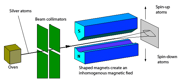
A diagram of the Stern-Gerlach experiment. Source: The Information Philosopher
Repeated measurements of spin
We saw previously that all three spin operators don't commute with each other; for instance, $[\hat S_x, \hat S_y] = i\hbar \hat S_z$. This is not just a mathematical peculiarity! In quantum mechanics, remember that any two operators that do not commute represent observables that cannot be simultaneously measured to arbitrary precision. In formal terms, the uncertainty principle tells us that for two non-commuting operators $\hat A, \hat B$, where $[\hat A, \hat B] = i\hat C$, then:
$$ \Delta A \Delta B \geq \dfrac{|\langle \hat C\rangle|}{2} $$
For instance, in the case of the position and momentum operators (where $[\hat x, \hat p] = i\hbar$), this reduces to the famous Heisenberg uncertainty principle:
$$ \Delta x \Delta p \geq \frac{\hbar}{2} $$
The consequence of the uncertainty principle is that if you measure one observable $A$ and then measure another observable $B$, if $\hat A, \hat B$ do not commute, then:
- They cannot both be measured simultaneously to perfect accuracy, and
- A measurement of one observable tells you nothing about the other observable
Let's break down what this means. Suppose you had an electron which initially is know to be spin-up along $z$. Mathematically, you know the precise value of the $\hat S_z$ operator (spin operator in the z direction): there is 100% probability that the electron is in the spin-up state along the $z$ axis. What happens if you measure the electron's spin along $x$? Well, the electron is equally likely to be spin-up or spin-down along the $x$ axis because of rule (2). We already saw that $[\hat S_z, \hat S_x] \neq 0$ (that is, the spin operators along $z$ and $x$ do not commute), so knowing $S_z$ (the electron's spin along $z$) tells you nothing about $S_x$.
Now, what happens if you measure the electron's spin along $z$ again? "This is a pointless question!", you may say, "since I already measured the electron to be in the spin-up state along $z$, so it must certainly be in that same state!" However, things are not quite so simple. Remember that since the spin operators along $z$ and $x$ do not commute, measuring $S_x$ tells you nothing about $S_z$ (and vice-versa). This means that if you know $S_x$, you would not know anything about $S_z$ prior to measuring it. Since you had measured $S_x$, if you then choose to measure $S_z$, it would be a contradiction if the electron's spin along $z$ could also be precisely known to be in one state. Thus we are left with the profound and puzzling conclusion that upon measuring $S_z$ after $S_x$, the electron is again equally likely to be spin-up or spin-down along the $z$ axis. The previous information you had about the electron - namely, that it was in the spin-up state along $z$ - has now been erased!
Larmor precession
If we think about a spinning top rotating on a table, it will rotate round and round in a circle tilted at an angle (until it inevitably falls). This phenomenon is known as precession, and is shown in the animation below:
Source: Wikimedia Commons
The reason why everyday precession happens is that the Earth's gravity produces a torque on the spinning top. But since it is also spinning, the top has angular momentum which resists the torque, leading to the gyroscope rotating at an angle. In physics, the gyroscope is said to precess. But angular momentum is not just found in the classical world: it is also found in the quantum world, and it leads to an effect called Larmor precession.
To understand Larmor precession, recall that we earlier noted that spin-1/2 particles have an intrinsic angular momentum that comes from their spin. We have notated this angular momentum as $\mathbf{S}$, as it is the spin angular momentum, and we know it must have a magnitude of $\pm \hbar/2$ along any axis (so long as it is a spin-1/2 particle). This angular momentum creates a magnetic moment $\vec{\boldsymbol{\mu}}$ associated with the particle, given by:
$$ \vec{\boldsymbol{\mu}} = \gamma \mathbf{S} $$
Here, $\gamma$ is known as the gyromagnetic ratio, and it is a constant that can be calculated from the mass, charge, and other characteristics of the particle in question. From the magnetic moment, we can construct a Hamiltonian for a spin-1/2 particle placed in an applied magnetic field $\mathbf{B}$ with the spin operator $\mathbf{\hat S}$, given by:
$$ \hat H = -\vec{\boldsymbol{\mu}} \cdot \mathbf{B} = -\gamma(\mathbf{\hat S} \cdot \mathbf{B}) $$
It is usually easiest to consider a magnetic field aligned along the $z$-direction, and thus we have:
$$ \hat H = -\gamma \hat S_z B_z $$
By solving for the eigenvalues and eigenstates of the Hamiltonian, we get two spin eigenstates, which are respectively given by:
$$ |\uparrow_z\rangle = \begin{pmatrix} 1 \\ 0 \end{pmatrix},\quad |\downarrow_z\rangle = \begin{pmatrix} 0 \\ 1 \end{pmatrix} $$
Meanwhile, the energy eigenvalues are given by:
$$ E_{\pm z} = \pm \frac{1}{2}\hbar \gamma B_z $$
This tells us that we have two distinct energy eigenstates: the first one with higher energy, and the second one with lower energy. The energy difference between the two energy levels can be written in terms of the Larmor frequency $\omega_0$ via:
$$ \begin{align*} \Delta E &= E_+ - E_- \\ &= \hbar \gamma B_z \\ &= \hbar \omega_0, \quad \omega_0 \equiv |\gamma B_z| \end{align*} $$
Physically, when a magnetic field is applied, we say that the magnetic moments of a spin-1/2 particle precess, since they rotate (just like a gyroscope) to line up along or against the magnetic field. This type of precession is called Larmor precession, and it is very similar to the classical precession of a gyroscope, with some notable differences being that there is nothing physically "rotating" at an angle; rather, it is the magnetic moment vector that becomes tilted off-axis, which is why we term it as precession.

A diagram of Larmor precession. Source: Wikimedia Commons
Precise measurements of Larmor precession are essential in many areas of science, especially in nuclear magnetic resonance (NMR) spectroscopy, which is used in the medical sciences, as well as biotechnology and biochemistry. Additionally, many electronic devices (like hard disk storage) relies on exploiting the effects of spin, with an entire field of [spintronics](https://en.wikipedia.org/wiki/Spintronics devoted to research in this area. With so many observations proving the existence of spin, we know for certain that even if spin runs counter to our intuitions (pun intended!), it is nevertheless a very real aspect of the quantum world.
Generalized two-level systems
We will close our introductory discussion of spin and the ways to analyze spin by quickly discussing the generalization of a spin-1/2 system: two-level systems. Two-level systems (that is, a quantum system with two degrees of freedom) are found throughout quantum mechanics. Since spin-1/2 particles can either be spin-up or spin-down, which are the only two possible states in a spin-1/2 system, it is the prototypical two-level system. However, it is by no means unique: there are other two-level systems out there, and they can often be modelled using the same tools. For instance, it is very common to see Hamiltonians of the form:
$$ \hat H \propto \sigma_i $$
Where $\sigma_i \in [\sigma_x, \sigma_y, \sigma_z]$ is a Pauli matrix, and they obey:
$$ \begin{align*} [\sigma_x, \sigma_y] = \sigma_z \\ [\sigma_y, \sigma_z] = \sigma_x \\ [\sigma_z, \sigma_x] = \sigma_y \end{align*} $$
The Bloch sphere
A common generalization of the spin-1/2 system we have discussed at length is known as the Bloch sphere. The Bloch sphere is a formulation of a generalized two-level system with two states, which we notate as $|0\rangle$ and $|1\rangle$. Here, $|0\rangle$ is the ground state, so it is associated with a lower energy, whereas $|1\rangle$ is the excited state, so it is associated with a higher energy.
The Bloch sphere (illustrated in the diagram below) allows us to visualize the abstract space in which these states "live", much like the complex plane can be drawn as a 2D coordinate grid. The state space of the system is parametrized in spherical coordinates by the angles $(\theta, \phi)$ - it is important to note that these aren't physical locations in space, but are rather located in the abstract Hilbert space of the two-state system.

An illustration of the Bloch sphere. Source: Wikipedia
On the Bloch sphere, $|0\rangle$ "lives" at the north pole of the Bloch sphere, and $|1\rangle$ "lives" at the south pole. Other states of the system lie somewhere between the two poles. The general state-vector of the system can thus be written as:
$$ |\psi\rangle = \cos\left( \frac{\theta}{2} \right) |0\rangle + e^{i\phi} \sin\left( \frac{\theta}{2} \right) |1\rangle $$
Where $e^{i\phi}$ is the phase of the state-vector, and where the basis states are given by:
$$ |0\rangle = \begin{pmatrix} 1 \\ 0 \end{pmatrix}, \quad |1\rangle = \begin{pmatrix} 0 \\ 1 \end{pmatrix} $$
Note: in the standard convention, the $x$ axis represents the real part of the phase, whereas the $y$ axis represents the imaginary part of the phase.
In the case that the two-level system models a spin-1/2 particle (a very common but not universal case), then we have:
$$ |\psi\rangle = \cos\left( \frac{\theta}{2} \right) |\uparrow\rangle + e^{i\phi} \sin\left( \frac{\theta}{2} \right) |\downarrow\rangle $$
Note: the choice is mathematically-arbitrary, so it does not matter whether we call $|0\rangle$ the spin-up or spin-down state, as long as our choice is consistent. However, $|\uparrow\rangle$ is usually associated with $|0\rangle$ in physics and engineering, and likewise $|\downarrow\rangle$ is usually associated with $|1\rangle$.
Along the "equator" of the Bloch sphere, we have $\theta = \pi/2$, and thus the state-vector takes the simpler form:
$$ |\psi\rangle = \frac{1}{\sqrt{ 2 }}\big(|0\rangle + e^{i\phi}|1\rangle\big) $$
Note that this corresponds to a state with 50% probability of measuring $|0\rangle$ and $|1\rangle$ since the complex phase factor has unit magnitude (you can check it for yourself by computing $P_0 = |\langle 0|\psi\rangle|^2$ and $P_1 = |\langle 1|\psi\rangle|^2$). However, the phase is still physically-relevant
Hamiltonian of a generalized two-level system
A very common basic Hamiltonian for a generalized two-level system is given by:
$$ \hat{H} = \frac{\hbar \omega}{2} \sigma_{z} $$
The energy eigenvalues are then $E = \pm \frac{1}{2} \hbar \omega$, with an energy difference of $\Delta E = \hbar \omega$ between the ground state and the excited state. Thus, the general time-dependent state-vector of the system, valid for all $t$, is given by:
$$ |\psi(t)\rangle = \cos\left( \frac{\theta}{2} \right) |0\rangle e^{-i \omega t/2} + e^{i\phi} \sin\left( \frac{\theta}{2} \right) |1\rangle e^{i \omega t/2} $$
This comes from tacking on a factor of $e^{-i E t/\hbar}$ to each of the eigenstates, and substituting in our known values of $E = \pm \frac{1}{2}\hbar\omega$. It is standard to factor out the phase factor of $e^{-i\omega t/2}$, giving us:
$$ \begin{align*} |\psi(t)\rangle &= e^{-i \omega t/2}\left[\cos\left( \frac{\theta}{2} \right) |0\rangle + e^{i\phi} \sin\left( \frac{\theta}{2} \right) |1\rangle e^{i \omega t} \right] \\ &= e^{-i \omega t/2}\left[\cos\left( \frac{\theta}{2} \right) |0\rangle + e^{i(\phi + \omega t)} \sin\left( \frac{\theta}{2} \right) |1\rangle\right] \end{align*} $$
Since the factor $e^{-i\omega t/2}$ is a phase factor, its magnitude is one, and thus it is not directly observable; thus, the physics of the system are identical if it is dropped. Defining $\phi_{r}(t) = \phi + \omega t$ as the relative phase of the system (since it is a phase that comes from the difference in energy of the two states, which is a relative quantity), we can rewrite the state-vector as:
$$ |\psi(t)\rangle = \cos\left( \frac{\theta}{2} \right) |0\rangle + e^{i\phi_{r}(t)} \sin\left( \frac{\theta}{2} \right) |1\rangle $$
As long as the system is undisturbed and the Hamiltonian is time-independent, the relative phase $\phi_r$ changes by a constant rate $\omega$ (the Larmor frequency) as the state-vector precesses along the Bloch sphere - note this is independent of the $\theta$ coordinate! If we imagine the state-vector of the system to be represented by an arrow, the change in the relative phase can be visualized as the rotation of this "arrow" as it precesses (i.e. rotates) around the Bloch sphere.
Note: For an application of the Bloch sphere in quantum optics, please see these lecture notes.
Conclusion to two-level systems
Two-level systems are the fundamental model behind a vast variety of quantum systems, including qubits in quantum computing, optically-pumped lasers, and molecular ions, as well as playing an important role in understanding the emission and absorption of radiation at the quantum level. We will discuss more examples of them throughout this guide - stay tuned!
The quantum harmonic oscillator
One of the simplest, but most important quantum systems is the quantum harmonic oscillator. At face value, it describes a particle in a harmonic potential well. To start, let us recall that the classical harmonic potential is given by:
$$ V(x) = \dfrac{1}{2} kx^2 = \dfrac{1}{2} m\omega^2 x^2, \quad \omega \equiv \sqrt{k/m} $$
The classical solutions to the (classical) harmonic oscillator are in terms of sinusoidal functions, which is why it is indeed called the harmonic oscillator. However, on a basic level, a harmonic potential is nothing more than a basic quadratic potential, one that we show in the below diagram:

In quantum mechanics, we retain the same form of the harmonic potential, except we perform the substitution $x \to \hat x$, where $\hat x$ is the position operator. Thus the Hamiltonian is given by:
$$ \hat H = \dfrac{\hat p^2}{2m} + V(x) = \dfrac{\hat p^2}{2m} + \dfrac{1}{2} m\omega^2 \hat x^2 $$
Note that we can also write this in the position representation (where $\hat x = x$ and $\hat p = -i\hbar \frac{d}{dx}$ in 1D) as:
$$ \hat H = -\frac{\hbar^2}{2m} \dfrac{d^2}{dx^2} + \frac{1}{2} m \omega^2 x^2 $$
The quantum harmonic oscillator is a very useful model in quantum mechanics, since it is one of the few problems that can be solved exactly. This does not mean it is trivial - the quantum harmonic oscillator finds numerous applications in molecular and atomic physics. The quantum harmonic oscillator can first be used as an approximation for a complicated potential. This is because the Taylor expansion of an arbitrary potential centered at $x = x_0$ is given by:
$$ V(x) = V_0 + V'(x-x_0) + \dfrac{1}{2} V''(x-x_0)^2 + \dfrac{1}{6} V'''(x-x_0)^3 + \dots $$
Another application is to describe the interaction of a charged (quantum) particle with an standing electromagnetic waves, something we will discuss later. When an electromagnetic field is trapped in some cavity, it decomposes into a series of modes, whose wavelength can only come in quantized values:
$$ \omega = \dfrac{2\pi c}{\lambda}, \quad \lambda = \dfrac{2L}{n}, \quad n = 1,2,3, \dots $$
Thus, any charged particle within such a cavity will interact with the standing waves of the electromagnetic field, leading to its energy levels being quantized. This is the origin of uniquely quantum phenomena such as the Stark effect, but we'll explain this in more detail later.
The third main application of the quantum harmonic oscillator is to describe the interaction of a particle with a quantized electromagnetic field, which is the realm of quantum electrodynamics and second quantization. While this can get complicated very quickly, the essence is to describe the quantized electromagnetic field as a series of coupled harmonic oscillators. We will cover this more at the very end of this guide.
To solve the quantum harmonic oscillator we begin with the same general methods as for essentially any quantum system - to write out the eigenvalue equation for the Hamiltonian:
$$ \hat H|\psi\rangle = E|\psi\rangle $$
This is the starting point, and there are several different ways to proceed from here. For instance, we can solve the eigenvalue equation in the position basis by taking the inner product with a position basis ket:
$$ \begin{gather*} \langle x|\hat H|\psi\rangle = \langle x|E|\psi\rangle \\ \langle x|\hat H|\psi\rangle = E\langle x|\psi\rangle \\ \left\langle x \left|-\dfrac{\hbar^2}{2m}\dfrac{d^2}{dx^2} + \dfrac{1}{2} m\omega^2 \hat x^2\right|\psi\right\rangle = E\langle x|\psi\rangle \\ \Rightarrow -\dfrac{\hbar^2}{2m}\dfrac{d^2 \psi}{dx^2} + \dfrac{1}{2} m\omega^2 x^2 \psi(x) = E \psi(x) \end{gather*} $$
This is a differential equation that can indeed be solved, although it is not very easy to solve. Indeed, a much better approach is to use the so-called algebraic approach, which originated with the physicist Paul Dirac, which we'll now discuss.
The ladder operator approach
Dirac's key insight in solving the quantum harmonic oscillator is to "factor" the Hamiltonian by defining two new operators $\hat a$ and $\hat a^\dagger$, given by:
$$ \begin{align*} \hat a &= \dfrac{1}{\sqrt{2}}(\hat x'+ i\hat p') \\ \hat a^\dagger &= \dfrac{1}{\sqrt{2}}(\hat x' - i\hat p') \end{align*} $$
Where $\hat x', \hat p'$ are related to the position and momentum operators $\hat x, \hat p$ as follows:
$$ \hat x' = \sqrt{\dfrac{m\omega}{\hbar}} \hat x, \quad \hat p' = \dfrac{1}{\sqrt{m\hbar \omega}} \hat p $$
It is also useful to note that:
$$ \begin{align*} \hat x' &= \frac{1}{\sqrt{2}}(\hat a^\dagger + \hat a) \\ \hat p' &= \dfrac{i}{\sqrt{2}}(\hat a^\dagger - \hat a) \\ \end{align*} $$
$\hat a$ and $\hat a^\dagger$ are conventionally called the ladder operators. These two operators satisfy $[\hat a, \hat a^\dagger] = 1$, an important identity to keep in mind for later. While many steps avoid using this approach and write $\hat a$ and $\hat a^\dagger$ purely in terms of $\hat x$ and $\hat p$, by defining our new operators $\hat x', \hat p'$ we can non-dimensionalize the problem, making it easier to solve. This is essentially the same thing as a change of variables in a classical mechanics problem, only here we're using operators, not classical functions.
Note: While $\hat a$ and $\hat a^\dagger$ are indeed adjoints of each other, it is common to consider them essentially separate operators (for reasons we'll soon see). It is also common to use the notation $(\hat a_-, \hat a_+)$ instead of $(\hat a, \hat a^\dagger)$ (where $\hat a_- = \hat a$ and $\hat a_+ = \hat a^\dagger$) which is a completely equivalent notation.
Thus, with our operators $\hat x'$ and $\hat p'$, the Hamiltonian can be written as:
$$ \hat H = \hbar \omega \hat H', \quad \hat H' = \dfrac{1}{2}(\hat x'^2 + \hat p'^2) $$
These operators allow us to simplify the Hamiltonian down greatly, since we find that:
$$ \begin{align*} \hbar \omega\left(\hat a^\dagger \hat a + \frac{1}{2}\right) &= \hbar \omega\left(\frac{1}{2}(\hat x' + i\hat p')(\hat x' - i\hat p') + \frac{1}{2}\right)\\ &= \dfrac{1}{2}\hbar \omega \left(\hat x'^2 - i\hat x' \hat p' + i\hat x' \hat p' + \hat p'^2 + 1\right) \\ &= \dfrac{1}{2}\hbar \omega(\hat x'^2 + \hat p'^2 + i[\hat x', \hat p'] + 1) \\ &= \dfrac{1}{2}\hbar \omega(\hat x'^2 + \hat p'^2 -1 + 1) \\ &= \hbar \omega H' \\ &= \hat H \end{align*} $$
If one defines another new operator $\hat N$ (we will discuss what this means later), given by $\hat N = \hat a^\dagger \hat a$, then the Hamiltonian takes the form:
$$ \hat H = \hbar \omega \left(\hat N + \dfrac{1}{2}\right) $$
Note: Be careful of the order of the $\hat a$ and $\hat a^\dagger$ operators! This is because $\hat N = \hat a^\dagger \hat a$, but $\hat a^\dagger \hat a \neq \hat a \hat a^\dagger$ so $\hat N \neq \hat a \hat a^\dagger$! Indeed we find that $\hat a \hat a^\dagger = 1 + \hat N$, which can be derived from the commutation relation $[\hat a, \hat a^\dagger] = 1$.
The genius of using this operator-based "algebraic" approach to solving the quantum harmonic oscillator is that the $\hat a, \hat a^\dagger$ operators satisfy:
$$ \hat a|\psi_0\rangle = 0, \quad \hat a^\dagger |\psi_0\rangle = |\psi_1\rangle $$
In fact, in the general case, we find that for the $n$-th eigenstate $|\psi_n\rangle$ we have:
$$ \hat a|\psi_n\rangle = \sqrt{n}|\psi_{n - 1}\rangle, \quad \hat a^\dagger|\psi_n\rangle = \sqrt{n + 1}~|\psi_{n + 1}\rangle $$
It is common convention to indicate the $n$-th eigenstate of the quantum harmonic oscillator with $|n\rangle = |\psi_n\rangle$, in which case one may write the more elegant expression:
$$ \hat a|n\rangle = \sqrt{n}~|n-1\rangle, \quad \hat a^\dagger|n\rangle = \sqrt{n+1}~|n + 1\rangle $$
Thus we again find that $\hat a|0\rangle = \hat a|\psi_0\rangle = 0$ and $\hat a^\dagger |0\rangle = \hat a|\psi_0\rangle = |\psi_1\rangle$. These are indeed the chief identities of the quantum harmonic oscillator, because if we substitute in the definitions of the $\hat a, \hat a^\dagger$ operators, we have:
$$ \begin{align*} \hat a^\dagger \hat a|n\rangle &= \hat a^\dagger(\sqrt{n}~|n+1\rangle) \\ &= \sqrt{n^2} |(n + 1) - 1\rangle \\ &= n|n\rangle \end{align*} $$
But we already know that $\hat a^\dagger \hat a$ is just the $\hat N$ operator, so we therefore have:
$$ \hat N|n\rangle = n|n\rangle $$
In addition, we have:
$$ \begin{align*} \hat a^\dagger\hat a|n\rangle &= \hat N|n\rangle = n|n\rangle \\ \hat a \hat a^\dagger|n\rangle &= (\hat N + \hat I)|n\rangle = (n + 1)|n\rangle \end{align*} $$
The $\hat N$ operator is often called the number operator since it returns the index $n$ corresponding to the nth eigenstate. For instance, for the first eigenstate $|0\rangle$ (in more traditional notation, this can be written as $|\psi_0\rangle$, which is equivalent), $\hat N|0\rangle = 0$, which tells us that (as we expect) the first eigenstate is labelled with index $n = 0$. Likewise, for the eigenstate $|3\rangle$ then $\hat N|3\rangle = 3 |n\rangle$, which indeed returns its index $n = 3$. What makes it particularly special is how the number operator can be defined solely in terms of the $\hat a$ and $\hat a^\dagger$ operators, which is a very non-trivial result. Thus, if we substitute $\hat N|n\rangle = n|n\rangle$ into our Hamiltonian, we have:
$$ \hat H|n\rangle = \hbar \omega \left(\hat N + \dfrac{1}{2}\right)|n\rangle = \underbrace{\hbar \omega \left(n + \dfrac{1}{2}\right)}_{E_n}|n\rangle $$
Where by comparison our expression with the Hamiltonian's eigenvalue equation $\hat H|n\rangle = E_n|n\rangle$, we find that:
$$ E_n = \hbar \omega\left(n + \dfrac{1}{2}\right) $$
Thus, we have found the energy eigenvalues without needing to solve any differential equation, which is quite an enormous feat! Additionally, since the energies are only dependent on $n$, the energies are non-degenerate, meaning that each energy eigenvalue is associated with a distinct eigenstate. This is incredibly important because it's uncommon to encounter fully non-degenerate systems in quantum mechanics, where each eigenstate can be labelled by a single eigenvalue (think about our previous discussion of CSCOs).
In addition, we can also calculate the eigenstates in the position (or momentum) bases, so the algebraic formalism helps us get the wavefunctions too. To do so, let us recognize that if we take the $n = 0$ state (often called the ground state, and notated as $|0\rangle$), we have $\hat a |0\rangle = 0$. Keep this in mind! Now, recall that we defined our relevant operators to take the following forms:
$$ \begin{align*} \hat a &= \dfrac{1}{\sqrt{2}}(\hat x'+ i\hat p') \\ &= \sqrt{\dfrac{m\omega}{2\hbar}}\hat x + \frac{i}{\sqrt{2m\omega \hbar}}\hat p \\ \hat a^\dagger &= \dfrac{1}{\sqrt{2}}(\hat x' - i\hat p') \\ &= \sqrt{\dfrac{m\omega}{2\hbar}}\hat x + \frac{i}{\sqrt{2m\omega \hbar}}\hat p \end{align*} $$
Thus, the explicit forms of $\hat a$ and $\hat a^\dagger$ can be found in the position basis by substituting in $\hat x = x$ and $\hat p = -i\hbar \dfrac{d}{dx}$, giving us:
$$ \begin{align*} \hat a &= \sqrt{\frac{m\omega}{2\hbar}} \left(x + \frac{\hbar}{m\omega} \dfrac{d}{dx}\right) \\ \hat a^\dagger &= \sqrt{\frac{m\omega}{2\hbar}} \left(x - \frac{\hbar}{m\omega} \dfrac{d}{dx}\right) \end{align*} $$
Now substituting these the explicit form of $\hat a$ in the position basis, we have:
$$ \begin{gather*} \hat a|0\rangle = 0 \\ \Rightarrow ~ \hat a\langle x|0\rangle = \hat a\psi_0(x) = 0 \\ \Rightarrow ~ \left(x + \dfrac{\hbar}{m\omega} \dfrac{d}{dx}\right)\psi_0(x) = 0 \end{gather*} $$
Note: It is also possible to do this in the momentum basis but the calculations become much more hairy. See this Physics StackExchange answer if interested.
This gives us a differential equation to solve, albeit a much easier one that can be solved explicitly by the standard methods of solving 1st-order differential equations. The solution is a Gaussian function, and in particular:
$$ \psi_0(x) = C e^{-m\omega x^2 / (2\hbar)} $$
And applying the normalization condition, the undetermined constant $C$ can be found to be $C = \left(\frac{m\omega}{\pi \hbar}\right)^{1/4}$, and thus we have:
$$ \psi_0(x) = \left(\dfrac{m\omega}{\pi \hbar}\right)^{1/4} e^{-m\omega x^2 / (2\hbar)} $$
Note: Since this is a Gaussian function, it is thus symmetric about $x = 0$, and thus we can infer that the expectation value of $\psi_0(x)$ (the quantum harmonic oscillator in its ground state) is $\langle x\rangle = 0$, which is also true for the classical harmonic oscillator.
We can then use the definition of the $\hat a^\dagger$ operator to find all of the wavefunctions for the higher-energy states, since:
$$ \begin{gather*} \hat a^\dagger|n\rangle = \sqrt{n + 1}~|n+1\rangle \\ \Rightarrow ~ \hat a^\dagger\langle x|n\rangle = \sqrt{n + 1}\langle x|n+1\rangle \\ \Rightarrow ~ \hat a^\dagger \psi_n(x) = (\sqrt{n + 1} )~\psi_{n + 1}(x) \end{gather*} $$
Thus, we have:
$$ \begin{align*} \psi_{n + 1}(x) &= \dfrac{1}{\sqrt{n + 1}} \hat a^\dagger \psi_n(x) \\ &= \psi_{n + 1}(x) \\ &= \ \sqrt{\frac{m\omega}{2(n+1)\hbar}} \left(x - \frac{\hbar}{m\omega} \dfrac{d}{dx}\right) \psi_n(x) \end{align*} $$
This allows us to recursively construct all the eigenstates of the system. For instance, we have:
$$ \begin{align*} \psi_1(x) &= \dfrac{1}{\sqrt{0 + 1}}\hat a^\dagger \psi_0(x) \\ &= \ \sqrt{\frac{m\omega}{2\hbar}} \left(x - \frac{\hbar}{m\omega} \dfrac{d}{dx}\right) \left[\left(\frac{m\omega}{\pi \hbar}\right)^{1/4} e^{-m\omega x^2 / (2\hbar)}\right] \\ &= \left(\frac{m\omega}{\pi \hbar}\right)^{1/4} \sqrt{\frac{2m\omega}{\hbar}} \, x \, e^{-\frac{m\omega}{2\hbar}x^2} \\ &= \left(\dfrac{4m^3\omega^3}{\pi \hbar^3}\right)^{1/4} x e^{-m\omega x^2 / (2\hbar)} \end{align*} $$
In general, we have:
$$ \begin{gather*} |n\rangle = \dfrac{(\hat a^\dagger)^n}{\sqrt{n!}}|0\rangle, \\ \psi_n(x) = \langle x|n\rangle = \sqrt{\frac{m\omega}{2\hbar n!}} \left(x - \frac{\hbar}{m\omega} \dfrac{d}{dx}\right)^n \psi_0(x) \end{gather*} $$
In the same way, we can get $\psi_2$ from applying the $\hat a^\dagger$ operator on $\psi_1$, then get $\psi_3$ from $\psi_2$, then get $\psi_4$ from $\psi_3$, and so on and so forth. With some clever mathematics (that we won't show here), this recursive formula can be solved in closed-form to yield a generalized formula for the nth eigenstate's wavefunction representation:
$$ \psi_n(x) = \left(\dfrac{m\omega}{\pi \hbar}\right) \dfrac{1}{\sqrt{2^nn!}}H_n\left(\sqrt{\dfrac{m\omega}{\hbar}}x\right)\exp \left(-\dfrac{m\omega x^2}{2\hbar}\right) $$
Here, $H_n(x)$ is a Hermite polynomial of order $n$, defined as:
$$ H_n(x) = (-1)^n e^{x^2} \frac{d^n}{dx^n} e^{-x^2} $$
Where the first three Hermite polynomials are given by:
$$ \begin{align*} H_0(x) &= 1 \\ H_1(x) &= 2x \\ H_2(x) &= 4x^2 - 2 \end{align*} $$
Using these definitions, we show a plot of the ground-state wavefunction $\psi_0(x)$ and several excited states' wavefunctions below:
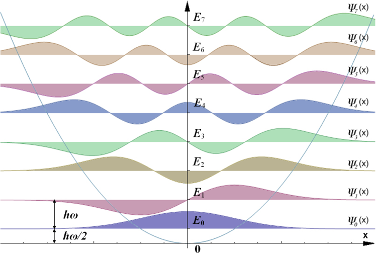
Source: Wikimedia Commons
We can also keep things abstract by noting that we can express any of the wavefunctions of each state $\psi_n(x)$ as $\psi_n(x) = \langle x|n\rangle$, where:
$$ |n\rangle = \dfrac{(\hat a^\dagger)^n}{\sqrt{n!}}|0\rangle, \quad \psi_0(x) = \langle x|0\rangle $$
The ladder operator approach to the quantum harmonic oscillator is a powerful technique, one that carries over to relativistic quantum mechanics and allows us to skip solving the Schrödinger equation entirely. In addition, solving problems using operators alone will give us the tools to understand the Heisenberg picture of quantum mechanics that we'll soon see.
Note for the advanced reader: The algebraic approach works mathematically because the eigenvalues of $\hat H$ are positive, and that the $\hat p^2$ operator is semi-positive definite. Additionally, the eigenspectrum (energy spectrum) of the system is discrete and non-degenerate (that is, all eigenstates have unique eigenvalues).
Expectation values of the quantum harmonic oscillator
In any quantum system, it is very useful to find their expectation values, and the same is true for the quantum harmonic oscillator. In particular, we are interested in calculating $\langle x\rangle$ and $\langle p\rangle$, the expectation values of the position and momentum. To do so, we will follow an approach from Brilliant wiki's authors. We start with the fact that:
$$ \begin{align*} \hat x' &= \frac{1}{\sqrt{2}}(\hat a^\dagger + \hat a) \\ \hat p' &= \dfrac{i}{\sqrt{2}}(\hat a^\dagger - \hat a) \\ \end{align*} $$
Now, we can express $\hat x'$ and $\hat p'$ in terms of $\hat x$ and $\hat p$ by simply rearranging the definitions of $\hat x'$ and $\hat p'$ from earlier:
$$ \begin{align*} \hat x' &= \sqrt{\dfrac{m\omega}{\hbar}} \hat x \\ \hat p' &= \dfrac{1}{\sqrt{m\hbar \omega}} \hat p \\ \end{align*} \quad \Rightarrow \quad \begin{align*} \hat x &= \sqrt{\dfrac{\hbar}{m\omega}}\hat x' \\ \hat p &= \sqrt{m\hbar \omega}\, \hat p' \end{align*} $$
Thus we have:
$$ \begin{align*} \hat x &= \sqrt{\frac{\hbar}{2 m \omega}} (a^{\dagger} + a)\\ \hat p &= i \sqrt{\dfrac{m \hbar \omega}{2}} (\hat{a}^{\dagger} - a) \end{align*} $$
From here, we can easily calculate the expectation values of $x$ and $p$. We'll start with the expectation value of $x$:
$$ \begin{align*} \langle x \rangle &= \langle n|\hat x|n\rangle \\ &= \langle n| \sqrt{\frac{\hbar}{2 m \omega}} (\hat a^{\dagger} + \hat a)|n\rangle \\ &= \sqrt{\frac{\hbar}{2 m \omega}} \big[\langle n|\hat a^\dagger|n\rangle + \langle n|\hat a |n\rangle\big] \\ &= \sqrt{\frac{\hbar}{2 m \omega}} \big[\sqrt{n + 1} \langle n|n+1\rangle + \sqrt{n}\langle n|n-1\rangle] \\ & = 0 \end{align*} $$
Where we used our definitions $\hat a^\dagger = \sqrt{n + 1} |n+1\rangle$, $\hat a = \sqrt{n} |n-1\rangle$ and also utilized the fact that any two eigenstates are orthogonal, that is, $\langle n|m\rangle = \delta_{mn}$, so $\langle n|n+1\rangle$ and $\langle n|n-1\rangle$ are both automatically zero. We can do the same thing with the momentum operator:
$$ \begin{align*} \langle p \rangle &= \langle n|\hat p|n\rangle \\ &= \langle n| i \sqrt{\dfrac{m \hbar \omega}{2}} (\hat a^{\dagger} - \hat a)|n\rangle \\ &= i \sqrt{\dfrac{m \hbar \omega}{2}} \big[\langle n|\hat a^\dagger|n\rangle - \langle n|\hat a |n\rangle\big] \\ &= i \sqrt{\dfrac{m \hbar \omega}{2}} \big[\sqrt{n + 1} \langle n|n+1\rangle - \sqrt{n}\langle n|n-1\rangle] \\ & = 0 \end{align*} $$
Note: The result that $\langle x\rangle = \langle p\rangle = 0$ only holds true for single eigenstates. It does not necessarily hold true in a superposition of states.
The same methods of calculation can be used to establish that:
$$ \begin{align*} \langle \hat x^2\rangle &= \dfrac{\hbar}{2m\omega}(2n + 1) \\ \langle \hat p^2 \rangle &= \dfrac{\hbar m\omega}{2}(2n + 1) \end{align*} $$
From the formula for the uncertainty of an observable $\Delta A = \sqrt{\langle A^2\rangle - \langle A\rangle^2}$ this tells us that:
$$ \Delta x \Delta p = \dfrac{\hbar}{2}(2n + 1) $$
Where for the ground state ($n = 0$) we have the minimum uncertainty:
$$ \Delta x \Delta p = \dfrac{\hbar}{2} $$
The quantum harmonic oscillator in higher dimensions
It is also possible to solve the quantum harmonic oscillator in higher dimensions. Indeed, consider the quantum harmonic oscillator along a 2D plane or a 3D box, where we can use Cartesian coordinates. Here, we do not actually need to do much more solving at all. The only difference is that rather than a single integer $n$, we need one integer $n$ for each coordinate. That is to say, for 2D we need two integers $n_x, n_y$, and for 3D we need three integers $n_x, n_y, n_z$ to describe all the eigenstates of the system. Therefore, the respective energy eigenvalues are:
$$ \begin{align*} E_{n_x, n_y}^{(2D)} &= \hbar \omega \left(n_x + n_y + \dfrac{1}{2}\right) \\ E_{n_x, n_y, n_z}^{(3D)} &= \hbar \omega \left(n_x + n_y + n_z + \dfrac{1}{2}\right) \end{align*} $$
Note that this means that we have degenerate eigenenergies, losing one of the key distinguishing features of the 1D quantum harmonic oscillator. In addition, the excited-state wavefunctions are unfortunately much more complicated for the 2D and 3D cases; we will restrict our attention to just the ground-state wavefunction. In $K$ dimensions, the ground-state wavefunction is given by:
$$ \psi_0(\mathbf{r}) = \left(\dfrac{m\omega}{\pi \hbar}\right)^{K/4} \exp\left(-\dfrac{m\omega}{2\hbar}r^2\right), \quad r = |\mathbf{r}| $$
Note that in 2D and 3D, we also have different cases, such as the quantum harmonic oscillator across a disk or in a spherical region. In these cases, the ground-state wavefunction exhibits polar and spherical symmetry respectively, so the general solutions are quite different from the 1D case. This is very important in nuclear and molecular physics, although we will not discuss it further here.
Note for the interested reader: If you are interested in further applications of the quantum harmonic oscillator, it can be used to model diatomic molecules like $\ce{N2}$ or $\ce{O2}$ and describe atomic nuclei with the nuclear shell model, as well as serving an important role in second quantization of light - something we'll see more of later.
Time evolution in quantum systems
In all areas of physics, we're often interested in how systems evolve. A system that depends on time is usually called a dynamical system, and at different points in time, the state of the system changes. Now, if we know that at some initial time $t_0$ a system is in a particular state $A$, and at some arbitrary later time $t$ is in another state $B$, the time evolution of the system describes how the system "gets" from $A$ to $B$.
Consider a very simple example: a particle moving along a line. Its state is described by a single variable - position - which we describe with $x$. In physics, we would describe the motion of this particle with a function $x(t)$, which is a trajectory. This trajectory is the time evolution of the system, because from a certain initial time $t_0$, we can calculate the particle's position at any future time $t$ with $x(t)$.
In quantum mechanics, we also see quantum systems exhibit time evolution. For instance, the state-vector may have an initial state $|\psi(t_0)\rangle$ at time $t = t_0$, and at some future time $t$ have the final state $|\psi(t)\rangle$. The question is, how does that initial state become the final state? The answer to that question is the time-evolution operator $\hat U(t, t_0)$, which satisfies:
$$ |\psi(t)\rangle = \hat U(t, t_0)|\psi(t_0)\rangle $$
That is to say, the time-evolution operator maps the system's state at an initial time $t_0$ to its future state at time $t$. But how does this all work? This is what we'll explore in this section.
Unitary operators
Before we go more in-depth into the time-evolution operator, we need to introduce the idea of a unitary operator. An arbitrary unitary operator $\hat U$ (forget about the time-evolution operator for now) satisfies two essential properties:
- $\hat U^{-1} = U^\dagger$, that is, its inverse is equal to its adjoint.
- $\hat U \hat U^{-1} = \hat U^{-1} \hat U = 1$, that is, multiplying a unitary operator by its adjoint gives the identity matrix. Together with the first rule, this automatically means that $\hat U \hat U^\dagger = \hat U^\dagger \hat U = 1$.
Note on notation: We will frequently use the shorthand $\hat I = 1$, where $\hat I$ is the identity matrix, when discussing operators, but remember that matrix multiplication always gives another matrix (and not the scalar number 1), so this is just a shorthand!
Note that unitary operator is not necessarily Hermitian - in fact, it usually isn't! So why do we care about a non-Hermitian operator when most of the operators we use in quantum mechanics are Hermitian? Well, if we act a unitary operator $\hat U$ on a (normalized) state-vector, we find that:
$$ (\hat U |\psi\rangle)^\dagger(\hat U |\psi\rangle) = \langle \psi |\hat U^\dagger \hat U|\psi\rangle = \langle \psi|\psi\rangle = 1 $$
This is the most important property of a unitary operator - it preserves the normalization of the state-vector! That is to say, acting $\hat U$ on $|\psi\rangle$ does not change its normalization $\langle \psi|\psi\rangle = 1$.
The unitary time-evolution operator
Now let's return back to the time-evolution operator. It is no accident that we denoted the time-evolution operator as $\hat U(t, t_0)$ and a unitary operator as $\hat U$. This is because the time-evolution operator is a unitary operator. It is indeed common to call the time-evolution operator the unitary time-evolution operator for this very reason! So from this point on, anytime you see $\hat U$, that means the time-evolution operator (unless otherwise stated).
Here is where the unitary nature of the time-evolution operator truly makes sense. This is because by knowing $\hat U \hat U^\dagger = \hat U^\dagger \hat U = 1$, and that $|\psi(t)\rangle = \hat U|\psi\rangle$, we also know that:
$$ \langle \psi(t)|\psi(t)\rangle = \langle \psi(t_0)|\hat U^\dagger\hat U(t, 0)|\psi(t_0)\rangle = \langle \psi(t_0)|\psi(t_0)\rangle = 1 $$
That is, if a state-vector $|\psi\rangle$ is normalized at $t = t_0$, it will continue to be normalized for all future times $t$, satisfying the normalization condition. This means that the time-evolution operator $\hat U$ automatically guarantees conservation of probability in a dynamical quantum system (a system that changes with time). Furthermore, we also add the requirement that the time-evolution operator must satisfy:
$$ \hat U(t_0, t_0) = 1 $$
This means that:
$$ \hat U(t_0, t_0)|\psi(t_0)\rangle = |\psi(t_0)\rangle $$
Therefore operating $\hat U$ on the state-vector returns the system in its initial state at $t = t_0$. This makes sense because at the initial time $t_0$, the system hasn't had any time to evolve, so acting the time-evolution operator on it does nothing but tell you the initial state!
Note: Another name for the unitary time-evolution operator is the propagator, which is common in advanced quantum mechanics. Later on in this guide, when we cover the path integral formulation of quantum mechanics, we'll speak of $\hat U$ as the propagator. Remember that whether we call $\hat U$ the unitary time-evolution operator or the propagator, we are referring to the same thing!
Now, we've spoken a lot about what the time-evolution operator $\hat U$ does, but how do we express it in explicit form? To be able to start, let's write out the Schrödinger equation in a special form. The most general form of the Schrödinger equation - at least, in the form we've generally seen - is given by:
$$ i\hbar \dfrac{\partial}{\partial t}|\psi(t)\rangle = \hat H|\psi(t)\rangle $$
But since $|\psi(t)\rangle = \hat U|\psi\rangle$, this can also be written as:
$$ i\hbar \dfrac{\partial}{\partial t}\hat U|\psi(t_0)\rangle = \hat H(\hat U|\psi(t_0)\rangle) $$
Since $|\psi(t_0)\rangle$ does not depend on time, we can factor it out from both sides, giving us:
$$ i\hbar \dfrac{\partial}{\partial t} \hat U = \hat H \hat U $$
Which can be written more explicitly as:
$$ i\hbar \dfrac{\partial}{\partial t} \hat U(t, t_0) = \hat H \hat U(t, t_0) $$
This is the essential equation of motion for the unitary operator. We'll now do something that may defy intuition but is actually mathematically sound. First, we'll temporarily drop the operator hats and not write out the explicit dependence on $t$ and $t_0$, giving us:
$$ i\hbar \dfrac{\partial U}{\partial t} = HU $$
Now, dividing by $i\hbar$ from both sides gives us:
$$ \dfrac{\partial U}{\partial t} = \frac{1}{i\hbar}HU = -\frac{i}{\hbar} HU $$
(Here we use the fact that $1/i = -i$, and $\dot U = \frac{\partial U}{\partial t}$). This now looks like a differential equation in the form $\dot U = -\frac{i}{\hbar} H U$! Solving this differential equation (using separation of variables) along with our known property $U(t_0) = 1$ gives us:
$$ U = e^{-i H (t - t_0)/\hbar} $$
Now, we can restore the operator hats and we can write the most general form of the time evolution operator:
$$ \hat U(t, t_0) = \exp\left(-\dfrac{i}{\hbar} \hat H (t - t_0)\right) $$
If we adopt the convention of choosing $t_0 = 0$, this gives us:
$$ \hat U(t) = \exp\left(-\dfrac{i}{\hbar} \hat H t\right), \quad \hat U(t) \equiv \hat U(t, 0) $$
Perhaps you might be inclined to answer with "You're wrong! What in the world is the exponential function of a matrix??" The way of making sense of this is to recognize that the exponential function can be defined in terms of a power series:
$$ e^X = \exp(X) = \sum_{n = 0}^\infty \dfrac{X^n}{n!} $$
Taking powers of a matrix is a perfectly acceptable operation, and therefore a term like $\hat H^n$ would raise no alarms, since $\hat H^n = \underbrace{\hat H \hat H \dots \hat H}_{n \text{ times}}$. This allows us to write $\hat U(t)$ in the form:
$$ \begin{align*} \hat U &= \sum_{n = 0}^\infty \frac{1}{n!}\left(-\dfrac{i}{\hbar} \hat H t\right) \\ &= 1 -\frac{i}{\hbar} \hat H t - \frac{1}{2\hbar^2} \hat H^2 t^2 + \dots \end{align*} $$
Usually, applying this definition is quite cumbersome (summing infinite terms is hard!) but if we truncate the series to just a few terms, we can often find a good approximation to the full series. For instance, if we truncate the series to first-order, we have:
$$ \hat U \approx 1 -\frac{i}{\hbar} \hat H t $$
Using this approximation can allow us to calculate the future state of a time-dependent quantum system with only knowledge of the Hamiltonian and the initial state. Of course, since we truncated the series, this calculation can yield only an approximate answer, but in some cases an approximate answer is enough. Thus, the time-evolution operator is the starting-point for perturbative calculations in quantum mechanics, where we can make successively more accurate approximations to the future state of a quantum system by invoking the time-evolution operator in series form, and taking only the first few terms.
The Heisenberg picture
Introducing the time-evolution operator has an interesting consequence: it allows us to calculate the future state of any quantum system from a known initial state "frozen" in time. This is because the initial state of a quantum system has not had time to evolve yet, so it is independent of time. In fact, it is possible to dispense with time-dependence in calculations almost completely, because it turns out that there is also a way to calculate the measurable quantities of quantum systems at any future point in time without needing to explicitly calculate $|\psi(t)\rangle$. This approach is known as the Heisenberg picture in quantum mechanics.
Consider the position operator $\hat X$ (we will use an uppercase $X$ here for clarity). Normally, this is a time-independent operator, since we know it is defined by $\hat X|\psi_0\rangle = x|\psi_0\rangle$, where $|\psi_0\rangle$ is a stationary state and $x$ is a position eigenvalue: notice here that time does not appear at all as a variable. Taking the inner product of both sides with the bra $\langle \psi_0|$ gives us the expectation value of the position:
$$ \langle \psi_0|\hat X |\psi_0\rangle = \langle \psi_0| x|\psi_0\rangle $$
Now, we want to find a time-dependent version of the position operator, which we'll call $\hat x_H(t)$, which also satisfies an eigenvalue equation:
$$ \hat X_H(t)|\psi(t)\rangle = x(t)|\psi(t)\rangle $$
Notice how our position eigenvalue is now time-dependent, because as the state of the system changes, the positions $x(t)$ also change. Our challenge will be able to write $\hat X_H(t)$ in terms of $\hat X$. How can we do so? Well, recall that $|\psi(t)\rangle = \hat U|\psi(t_0)\rangle$, and $|\psi(t_0)\rangle$ is the same thing as $|\psi_0\rangle$. Thus we can write:
$$ \hat X_H(t)|\psi(t)\rangle = \hat X\hat U|\psi_0\rangle $$
Now, let us take its inner product with the bra $\langle \psi(t)|$, which gives us:
$$ \langle \psi(t)|\hat X_H(t)|\psi(t)\rangle = \langle \psi(t) |x\hat U|\psi_0\rangle $$
We'll now use the identity that:
$$ |\psi(t)\rangle = \hat U |\psi_0\rangle \quad \Leftrightarrow \quad |\psi_0\rangle = \hat U^\dagger |\psi(t)\rangle $$
You can prove this rigorously, but it can be intuitively understood by recognizing that $\hat U^\dagger = \hat U^{-1}$, meaning that just as $\hat U$ evolves the system forwards in time, $\hat U^\dagger$ evolves the system backwards in time (the "inverse" direction in time). Hence acting $\hat U^\dagger$ on a system at some time $t$ returns it to its original state at some past time $t_0$. With the same result, we note that:
$$ \langle \psi(t)|\hat X_H(t)|\psi(t)\rangle = \langle \psi(t) |x\hat U|\psi_0\rangle = \langle \psi_0|\hat U^\dagger x \hat U|\psi_0\rangle $$
Thus by pattern-matching we have:
$$ \hat X_H(t) = \hat U^\dagger x \hat U = \hat U^\dagger \hat X \hat U $$
Notice that the latter result holds for all time $t$! We have indeed arrived at our expression for the time-dependent version of the position operator $\hat X_H(t)$:
$$ \hat X_H(t) = \hat U^\dagger \hat X \hat U $$
It is also common to say that $\hat X_H$ is the position operator in the Heisenberg picture. Unlike the Schrödinger picture that we've gotten familiar working with, the Heisenberg picture uses time-dependent operators that operate on a constant state-vector $|\psi\rangle = |\psi_{0}\rangle$. It is completely equivalent to the Schrödinger picture, but it is sometimes more useful, since we can dispense with calculating the state-vector's time evolution as long as we know the $\hat U$ operator, which can simplify (some) calculations. In the most general case, for any operator $\hat A$, its equivalent time-dependent version $\hat A_H$ in the Heisenberg picture is given by:
$$ \hat A_H(t) = \hat U^\dagger \hat A \hat U $$
If we don't know $\hat U$, it is also possible to calculate $\hat A_H$ via the Heisenberg equation of motion, the analogue of the Schrödinger equation in the Heisenberg picture:
$$ \dfrac{d}{dt} \hat{A}_{H}(t) = \frac{i}{\hbar}[\hat{H}, \hat{A}_{H}(t)] $$
A particularly powerful consequence of the Heisenberg picture is how easily it maps classical systems into a corresponding quantum system. For instance, the classical harmonic oscillator follows the equation of motion $\dfrac{d^2 x}{dt^2} + \omega^2 x = 0$, which has the (classical) solution:
$$ \begin{align*} x(t) &= a e^{-i\omega t} + a^* e^{i\omega t} \\ p(t) &= m \dfrac{dx}{dt} = b^*e^{-i\omega t} + be^{i\omega t}, \quad b =i\omega ma^* \end{align*} $$
Where $a, a^*$ here are some amplitude constants that can be specified by the initial conditions, and for generality, we assume that they can be complex-valued. Now, the Heisenberg picture tells us that if we want to find the corresponding quantum operators $\hat X_H(t), \hat p(t)$, all we have to do is to change our constants $a, a^*$ to operators $\hat a, \hat a^\dagger$ (same with $b, b^*$), giving us:
$$ \begin{align*} \hat X_H(t) &= \hat ae^{-i\omega t} + \hat a^\dagger e^{i\omega t} \\ \hat p(t) &= \hat be^{-i\omega t} + \hat b^\dagger e^{i\omega t}, \quad \hat b = i\omega m a^\dagger \end{align*} $$
Indeed, we can then identify $\hat a, \hat a^\dagger$ as just the ladder operators we're already familiar with from studying the quantum harmonic oscillator! In addition, we can also show that $\hat x$ satisfies a nearly identical equation of motion as the classical case ($\frac{d^2 x}{dt^2} + \omega^2 x = 0$), with the exception that the position function $x$ is replaced by the operator $\hat X_{H}$:
$$ \dfrac{d^2 \hat X_H(t)}{dt^2} + \omega^2 \hat X_H(t) = 0 $$
Notice the elegance correspondence between the classical and quantum pictures. By doing very little work, we have quantized a classical system, taking a classical variable ($x(t)$, representing a particle's position) and turning it ("promoting it") into a quantum operator $\hat X_{H}(t)$, a process formally called first quantization. This method will be essential once we discuss second quantization, where we take classical field theories and use them to construct quantum field theories. But we've not gotten to there yet! We'll save a more in-depth discussion of second quantization for later.
Note for the advanced reader: In second quantization, we essentially do the same thing as first quantization, but rather than quantizing the position (by taking the classical variable $x(t)$ and promoting it to an operator $\hat X_{H}$) we are interested in taking a classical field $\phi(x, t)$ and promoting it to an quantum field operator $\hat \phi$. Just as in first quantization, second-quantized fields follow the same equations of motion as their classical field analogues. In particular, the simplest type of quantum field (known as the free scalar field) obeys the equation $\partial^2_{t}\hat \phi - \nabla^2 \phi + m^2\phi = 0$, which is very similar to the harmonic oscillator equation of motion.
The correspondence principle and the classical limit
As we have seen, the Heisenberg picture makes it easy to show the intricate connection between quantum mechanics and classical mechanics, which is also known as the correspondence principle. The correspondence principle is essential because it explains why we live in a world that can be so well-described by classical mechanics, even though we know that everything in the Universe is fundamentally quantum at the tiniest scales. A key part of the correspondence principle is Ehrenfest's theorem, which is straightforward to prove from the Heisenberg picture. We start by writing down the Heisenberg equation of motion (which we introduced earlier), given by:
$$ \dfrac{d}{dt} \hat{A}_{H}(t) = \frac{i}{\hbar}[\hat{H}, \hat{A}_{H}(t)] $$
The Heisenberg equations of motion for the position and momentum operators $\hat X_{H}(t)$, $\hat P_{H}(t)$ are therefore:
$$ \begin{align*} \dfrac{d \hat X_H(t)}{dt} = \frac{i}{\hbar}[\hat{H}, \hat X_H(t)] \\ \dfrac{d \hat P_H(t)}{dt} = \frac{i}{\hbar}[\hat{H}, \hat P_H(t)] \end{align*} $$
If we take the expectation values for each equation on both sides, we have:
$$ \begin{align*} \left\langle\dfrac{d \hat X_H(t)}{dt}\right\rangle = \frac{i}{\hbar}\langle[\hat{H}, \hat X_H(t)]\rangle \\ \left\langle\dfrac{d \hat P_H(t)}{dt}\right\rangle = \frac{i}{\hbar}\langle[\hat{H}, \hat P_H(t)]\rangle \end{align*} $$
Now making use of the fact that $[\hat H, \hat X_{H}(t)] = -i\hbar \frac{\hat{P}_{H}}{m}$ and $[\hat H, \hat P_{H}(t)] = i\hbar \nabla V$ (we won't prove this, but you can show this yourself by calculating the commutators with $\hat H = \hat P^2/2m + V$) we have:
$$ \begin{align*} \left\langle\dfrac{d \hat X_H(t)}{dt}\right\rangle = \frac{\langle \hat{P}_{H}\rangle}{m} \\ \left\langle\dfrac{d \hat P_H(t)}{dt}\right\rangle = \langle -\nabla V\rangle \end{align*} $$
The first equation tells us that the expectation value of the position is equal to the expectation value of the momentum, divided by the mass. In the classical limit, this is exactly $\dot x = p/m$, which comes directly from the classical definition of the momentum $p = mv = m\dot x$! Meanwhile, the second equation tells us that the expectation value of the momentum is equal to $\langle -\nabla V\rangle$. This is (approximately) the same as Newton's second law $F = \frac{dp}{dt} = -\nabla V$. Thus, Ehrenfest's theorem says that at classical scales, quantum mechanics reduces to classical mechanics; this is why we don't observe any quantum phenomena in our everyday lives!
The interaction picture
Using Heisenberg's approach to quantum mechanics is powerful, but it often comes at the cost of needing to compute a lot of operators. The physicist Paul Dirac looked at the Heisenberg picture, and decided that there was a better way that would simplify the calculations substantially, while preserving all of the physics of a quantum system. His equivalent approach is known as the interaction picture, although it is often also called the Dirac picture (obviously after him).
We will quickly go over the interaction picture for the sake of brevity. Essentially, it says that we can split a quantum system into two parts - a non-interacting part and an interacting part. When we say "non-interacting", we mean a hypothetical system that is completely isolated from the outside world and is essentially in a Universe of its own. To do this, we write the Hamiltonian of the system as the sum of a non-interacting Hamiltonian $\hat H_0$ and an interaction Hamiltonian $\hat W$:
$$ \hat{H} = \hat{H}_{0} + \hat{W} $$
As with the Schrödinger picture, the state-vector of the system $|\psi(t)\rangle$ will depend on time. But here is where the interaction picture begins to differ from the Schrödinger picture. First, let us consider the time-evolution operator $\hat U_0(t, t_{0}) = e^{-i\hat H_0 (t-t_{0})/\hbar}$. Strictly-speaking, this time-evolution operator is only valid for the non-interacting part of the system, since it comes from $\hat H_0$, the non-interacting Hamiltonian. We will now define a modified state-vector $|\psi_I(t)\rangle$, which is related to the original state-vector of the system $|\psi(t)\rangle$ by:
$$ |\psi_{I}(t)\rangle = \hat U_{0}^{\dagger} |\psi(t)\rangle = e^{i \hat{H}_{0} (t - t_{0})/\hbar} |\psi(t)\rangle $$
We can of course also invert this relation to write $|\psi(t)\rangle$ in terms of $|\psi_I\rangle$, as follows:
$$ |\psi(t)\rangle = \hat U_{0} |\psi_{I}(t)\rangle = e^{-i \hat{H}_{0} (t - t_{0})/\hbar} |\psi_{I}(t)\rangle $$
We can write an arbitrary operator $\hat A$ in its interaction picture representation, which we will denote with $\hat A_I$, via:
$$ \hat{A}_{I}(t) = \hat U_{0}^{\dagger} \hat{A} \hat U_{0} = e^{i \hat{H}_{0} (t - t_{0})/\hbar} \hat{A} e^{-i \hat{H}_{0} (t - t_{0})/\hbar} $$
In addition, an operator's representation in the interaction picture follows the equation of motion:
$$ i\hbar\frac{d \hat{A}_{I}}{dt} = [\hat{A}_{I}, \hat{H}_{0}] $$
Our modified state-vector $|\psi_I(t)\rangle$ then satisfies the following equation of motion:
$$ i\hbar \frac{d}{dt}|\psi_{I}(t)\rangle = \hat{W}_{I}|\psi_{I}(t)\rangle $$
Where $\hat W_I = \hat U_{0}^{\dagger} \hat{W} \hat U_{0}$ is the interaction picture representation of the interaction Hamiltonian $\hat W$. What this means is that using the interaction picture, we can isolate the interacting parts of the system from the non-interacting parts of the system - something that isn't possible to do in the Heisenberg or Schrödinger pictures! The interacting part of the system follow the equation of motion we already presented for $|\psi_I(t)\rangle$, whereas the non-interacting part satisfies the equation of motion for $\hat U_0$:
$$ i\hbar \dfrac{\partial}{\partial t} \hat U_{0}(t, t_0) = \hat H_{0} \hat U_{0}(t, t_0) $$
Since these two equations of motion are completely decoupled from each other, we can solve for the interacting and non-interacting parts separately. Once we have successfully solved for $|\psi_I(t)\rangle$ and $\hat U_0$, the state-vector of the full system is just a unitary transformation away, since:
$$ |\psi(t)\rangle = \hat U_{0} |\psi_{I}(t)\rangle $$
The interaction picture is powerful because it allows us to describe a quantum system that undergoes very complicated interactions as if those interactions were not present, and simply "layer" the interactions on top. This is an idea essential to solving very complicated quantum systems, especially once we get to the topic of time-dependent perturbation theory in quantum mechanics. As an added bonus, it turns out that under certain circumstances it is possible to write out an exact series solution to solve for the interacting part of a system. As long as we assume that interactions are reasonably "small", we can convert the equation of motion for the interacting part of the system into an integral equation:
$$ \begin{gather*} i\hbar \frac{d}{dt}|\psi_{I}(t)\rangle = \hat{W}_{I}|\psi_{I}(t)\rangle \\ \downarrow \\ |\psi_{I}(t) = |\psi_{I}(t_{0})\rangle + \frac{1}{i\hbar} \int_{t_{0}}^t dt' W_{I}(t')|\psi_{I}(t')\rangle \end{gather*} $$
One can then write out a series solution that solves the integral equation, which is given by:
$$ \begin{align*} |\psi_{I}(t) = \bigg\{1 &+ \frac{1}{i\hbar} \int dt_{1} W_{I}(t_{1}) + \frac{1}{(i\hbar)^2}\int dt_{1} dt_{2} W_{I}(t_{1})W_{I}(t_{2}) \\ &+ \dots + \frac{1}{(i\hbar)^n} \int dt_{1}dt_{2} \dots dt_{n} W_{I}(t_{1})W_{I}(t_{2}) \dots W_{I}(t_{n})\bigg\}|\psi_{I}(t_{0})\rangle \end{align*} $$
This is the Dyson series. Right now, the Dyson series is unimportant to us, but it has a great deal of importance in analyzing scattering. We have already seen scattering-state solutions to the Schrödinger equation, like the case of the rectangular potential barrier. But quantum-mechanical scattering is far more broad, and the Dyson series provides us with a way to calculate very complex scattering interactions in a solvable way. In fact, this technique is so general that it is even used in quantum field theory!
Summary of time evolution
We have seen that there are three equivalent approaches to understanding the time evolution of the quantum system: the Schrödinger picture, Heisenberg picture, and interaction (or Dirac) picture. In the Schrödinger picture, operators are time-independent but states are time-dependent; in the Heisenberg picture, operators are time-dependent but states are time-independent; and finally, in the interaction picture, both are time-dependent. Each of these approaches has their own strengths and weaknesses, and they are useful in different scenarios. The key idea is that having these different approaches to describing quantum systems gives us powerful tools to solve these systems, even if we don't have to use them all the time.
Angular momentum
In quantum mechanics, we are often interested in central potentials, that is, potentials in the form $V = V(r)$. For instance, the hydrogen atom can be modelled by a Coulomb potential $V(r) \propto 1/r$, and a basic model of the atomic nucleus uses a harmonic potential $V(r) \propto r^2$.
Note: In case it was unclear, in central potential problems, $r = \sqrt{x^2 + y^2 + z^2}$ is the radial coordinate.
Due to the symmetry of such problems, it is often convenient to use a radially-symmetric coordinate system, like polar coordinates (in 2D) or cylindrical/spherical coordinates (in 3D). This leads to an interesting result - the conservation of angular momentum. A rigorous explanation of why this is the case requires Noether's theorem, which is explained in more detail in the classical mechanics guide. There are a few differences, however. For instance, while classical central potentials lead to orbits around the center-of-mass of a system, the idea of orbits is somewhat vague in quantum mechanics since the idea of probability waves "orbiting" doesn't really make sense. However, for ease of visualization (and also due to some historical reasons), it is still common to say that central potential problems in quantum mechanics have "orbits", and thus we conventionally call this associated type of angular momentum the orbital angular momentum, denoted $\mathbf{L}$.
In addition, a classical spinning object also has angular momentum, and likewise a quantum particle also does - again, this is why we say that electrons (and other spin-1/2 particles) have spin, since they do have angular momentum in the form of spin angular momentum. Since we know the relationship between the magnetic moment $\boldsymbol{\mu}$ and the spin angular momentum $\mathbf{S}$ (it is proportional to a factor of $\gamma$, the gyromagnetic ratio), we can rearrange to find $\mathbf{S}$:
$$ \boldsymbol{\mu} = \gamma \mathbf{S} \quad \Rightarrow \quad \mathbf{S} = \frac{\boldsymbol{\mu}}{\gamma} $$
It is important to recognize that spin angular momentum $\mathbf{S}$ is different from the orbital angular momentum $\mathbf{L}$. They, however, share one important similarity - they are both conserved quantities. This means they obey some similar behaviors. Additionally, the study of orbital angular momentum is extremely important for understanding some of the most important problems in quantum mechanics, so we will explore it in detail.
Stationary perturbation theory
Perturbation theory exists when we come upon a problem that is too complicated to solve exactly. These problems are often (but not always) variations of existing problems. For instance, we know the solution of the hydrogen atom, since that can be solved exactly, but it turns out that for the helium atom, which has just one more electron than the hydrogen atom, there is no analytical solution! In such cases, we typically resort to one of two options:
- Solve the system on a computer using numerical methods
- Find an approximate analytical solution
The second option is what we'll focus on here, since numerical methods in quantum mechanics is a topic broad enough for an entire textbook on its own. This approach - making calculations using approximations - is known as perturbation theory, and it allows us to solve many kinds of problems that cannot be solved exactly.
Note: Perturbation theory, despite its association with quantum mechanics, is actually a far more general technique for solving complicated differential equations (even those describing classical systems). For more information, see this excellent article on a classical application of perturbation theory.
First off, we should mention that there are two general kinds of perturbation theory in quantum mechanics: stationary perturbation theory, which (as the name suggests) applies only for stationary (time-independent) problems, and time-dependent perturbation theory, which applies for problems that explicitly depend on time. Right now, we'll be focusing on stationary perturbation theory; we'll get to the time-dependent version later. While there are notable differences, both types of perturbation theory use the same general method: a complicated system is approximated as a simpler, more familiar system with some added corrections (called perturbations). By computing these correction terms, we are then able to find an approximate solution to the system, even if there is no exact analytical solution.
A description of perturbation theory from XKCD.
Non-degenerate perturbation theory
We will first review the simplest type of stationary perturbation theory, known as non-degenerate perturbation theory, which applies to quantum systems without degeneracy (meaning that each eigenstate is uniquely specified by an energy eigenvalue of the Hamiltonian). It turns out that this is in many cases an overly simplified assumption, but the methods we will develop here will be extremely useful for our later discussion of degenerate perturbation theory that accurately describes a variety of real-world quantum systems.
The starting point in perturbation theory is to assume that the Hamiltonian of a complicated system can be written as a sum of a Hamiltonian $\hat H_0$ with an exact solution and a small perturbation $\hat{W}$, such that:
$$ \hat{H} = \hat{H}_{0} + \lambda\hat{W} $$
Note: Here $\hat H_0$ is known as the unperturbed Hamiltonian or free Hamiltonian. Also, it is common to write $\hat W$ without the operator hat, and it is also common to denote it as $V$ (confusingly). Be aware that in all cases, $W$ is an operator, not a function!
For instance, $\hat H_0$ might be the Hamiltonian of a free particle, or of the hydrogen atom, or the quantum harmonic oscillator. The key commonality here is that $\hat H_0$ must be the Hamiltonian of a simpler system that can be analytically solved. On top of $\hat H_0$ we add the perturbation $\hat W$, which represents the deviations (also called perturbations) of the system's Hamiltonian as compared to the simpler system. This perturbation is assumed to be small, so we scale it by a small number $\lambda$ (where $\lambda \ll 1$), giving us a term of $\lambda \hat W$. If we write out the Schrödinger equation for the system, we have:
$$ \hat{H}|\varphi_{n}\rangle = E_{n} |\varphi_{n}\rangle \quad \Rightarrow \quad (\hat{H}_{0} + \lambda\hat{W})\varphi_{n}\rangle = E_{n} |\varphi_{n}\rangle $$
Note that when we take the limit $\lambda \to 0$, the perturbation vanishes, and the Hamiltonian is exactly the unperturbed Hamiltonian $\hat H_0$. This is why perturbation theory is an approximation; it assumes that the simpler system's Hamiltonian $\hat H_{0}$ is already close enough to the more complicate system's Hamiltonian $\hat H$ that $\hat H_0$ can be used to approximate $\hat H$.
The key idea of perturbation theory is that we assume a series solution for $\hat{H}|\varphi_{n}\rangle = E_{n}|\varphi_{n}\rangle$. More accurately, we assume that we can write the solution in terms of a power series in powers of $\lambda$. Now, this assumption doesn't always work - in fact there are some systems where it doesn't work at all - but using this assumption makes it possible to find an approximate solution using analytical methods, which is "good enough" for most purposes. Remember, in the real world, it is impossible to measure anything to infinite precision, so having an approximate answer to a problem that is close enough to the exact solution is often more than sufficient to make testable predictions that align closely with experimental data.
But let's get back to the math. For our solution to be expressed as a power series in $\lambda$, we would write:
$$ \begin{align*} |\varphi_{n}\rangle &= \sum_{m = 0}^\infty \lambda^m|\varphi_{n}^{(m)}\rangle \\ &=|\varphi_{n}^{(0)}\rangle + \lambda|\varphi_{n}^{(1)}\rangle + \lambda^2|\varphi_{n}^{(2)}\rangle + \dots \end{align*} $$
Here, remember that $|\varphi_{n}\rangle$ is the exact solution to the system (representing all $n$ exact eigenstates of the complicated Hamiltonian $\hat H$), but $|\varphi_{n}^{(0)}\rangle, |\varphi_{n}^{(1)}\rangle, |\varphi_{n}^{(2)}\rangle, \dots$ are successive states whose sum converges to the exact eigenstates of the system. (For those who need a refreshed on power series please see the series and sequences guide). Be aware that the brackets $(1), (2), \dots$ are not exponents; rather they are labels for the successive sets of eigenstates (the first set of eigenstates, the second, the third, and so forth). By summing up infinitely many of these terms in the expansion of the Hamiltonian's eigenstates, we would in principle get the exact eigenstates of the complicated Hamiltonian.
In the same way, we assume that the system's energy eigenvalues $E_n$ can also be written as a power series in $\lambda$, given by:
$$ \begin{align*} E_{n} &= \sum_{m=0}^\infty \lambda^m E_{n}^{(m)} \\ &= E_{n}^{(0)} + \lambda E_{n}^{(1)} + \lambda^2 E_{{n}}^{(2)} + \dots \end{align*} $$
The first term in the expansion, $E_n^{(0)}$, as we'll see, are simply the energy eigenvalues of the unperturbed Hamiltonian $\hat H_0$. The subsequent terms $E_{n}^{(1)}$, $E_{n}^{(2)}$ are known as the first-order correction and second-order correction to the energy eigenvalues, since they respectively have coefficients of $\lambda^1$ and $\lambda^2$. By summing up infinitely many of these terms in the expansion of the energy, we would in principle get the exact energies.
Now, if we substitute our power series solution into the Hamiltonian's eigenvalue equation $\hat{H}|\varphi_{n}\rangle = E_{n}|\varphi_{n}\rangle$, we have:
$$ \begin{align*} (\hat{H}_{0} + \lambda \hat{W})(|\varphi_{n}^{(0)}\rangle &+ \lambda|\varphi_{n}^{(1)}\rangle + \lambda^2|\varphi_{n}^{(2)}\rangle + \dots) \\ &= (E_{n}^{(0)} + \lambda E_{n}^{(1)} + \lambda^2 E_{{n}}^{(2)} + \dots)(|\varphi_{n}^{(0)}\rangle + \lambda|\varphi_{n}^{(1)}\rangle + \lambda^2|\varphi_{n}^{(2)}\rangle + \dots) \end{align*} $$
Distributing the left-hand side gives us:
$$ \begin{align*} \hat{H}_{0}\bigg(|\varphi_{n}^{(0)}\rangle &+ \lambda|\varphi_{n}^{(1)}\rangle + \lambda^2|\varphi_{n}^{(2)}\rangle + \dots\bigg) + \lambda \hat{W}\bigg(|\varphi_{n}^{(0)}\rangle + \lambda|\varphi_{n}^{(1)}\rangle + \lambda^2|\varphi_{n}^{(2)}\rangle + \dots\bigg) \\ &= E_{n}^{(0)}\left(|\varphi_{n}^{(0)}\rangle + \lambda|\varphi_{n}^{(1)}\rangle + \lambda^2|\varphi_{n}^{(2)}\rangle + \dots\right) \\ &\qquad+ \lambda E_{n}^{(1)}\left(|\varphi_{n}^{(0)}\rangle + \lambda|\varphi_{n}^{(1)}\rangle + \lambda^2|\varphi_{n}^{(2)}\rangle + \dots\right)\\ &\qquad+ \lambda^2 E_{n}^{(2)}\left(|\varphi_{n}^{(0)}\rangle + \lambda|\varphi_{n}^{(1)}\rangle + \lambda^2|\varphi_{n}^{(2)}\rangle + \dots\right) \end{align*} $$
If we do some algebraic manipulation to group terms by powers of $\lambda$, we get:
$$ \begin{align*} % LHS of equation \hat{H}_{0}|\varphi_{n}^{(0)}\rangle &+ \lambda \left(\hat{H}_{0}|\varphi_{n}^{(1)}\rangle + \hat{ W}|\varphi_{n}^{(0)}\rangle\right) + \lambda^2\left(\hat{H}_{0}|\varphi_{n}^{(2)}\rangle + \hat{W}|\varphi_{n}^{(1)}\rangle\right) + \dots \\ &= % RHS of equation E_{n}^{(0)}|\varphi_{n}^{(0)}\rangle + \lambda\left(E_{n}^{(0)}|\varphi_{n}^{(1)}\rangle + E_{n}^{(1)}|\varphi_{n}^{(0)}\rangle\right) + \lambda^2 \left(E_{n}^{(0)}|\varphi_{n}^{(2)}\rangle + E_{n}^{(1)}|\varphi_{n}^{(1)}\rangle + E_{n}^{(2)}|\varphi_{n}^{(0)}\rangle\right) + \dots \end{align*} $$
Notice how each term on the left-hand side of the equation now corresponds to a term on the right-hand side with the same power of $\lambda$. Thus, by equating the quantities in the brackets for every power of $\lambda$, we get a system of equations to solve for each order of $\lambda$:
$$ \begin{align*} \mathcal{O}(\lambda^0):& \quad E_{n}^{(0)}|\varphi_{n}^{(0)}\rangle \\ \mathcal{O}(\lambda^1):& \quad \lambda \left(\hat{H}_{0}|\varphi_{n}^{(1)}\rangle + \hat{W}|\varphi_{n}^{(0)}\rangle\right) = \lambda\left(E_{n}^{(0)}|\varphi_{n}^{(1)}\rangle + E_{n}^{(1)}|\varphi_{n}^{(0)}\rangle\right) \\ \mathcal{O}(\lambda^2):& \quad \lambda^2\left(\hat{H}_{0}|\varphi_{n}^{(2)}\rangle + \hat{W}|\varphi_{n}^{(1)}\rangle\right) = \lambda^2 \left(E_{n}^{(0)}|\varphi_{n}^{(2)}\rangle + E_{n}^{(1)}|\varphi_{n}^{(1)}\rangle + E_{n}^{(2)}|\varphi_{n}^{(0)}\rangle\right) \\ & \qquad\vdots \\ \mathcal{O}(\lambda^n): &\quad \lambda^n\left(\hat{H}_{0}|\varphi_{n}^{(n)}\rangle + \hat{W}|\varphi_{n}^{(n-1)}\rangle\right) = \lambda^n\left( E_{n}^{(0)}|\varphi_{n}^{(n)}\rangle + \sum_{j = 1}^n E_{n}^{(j)} \left|\varphi_{n}^{(n - j)}\right\rangle\right) \end{align*} $$
Note: The final, generalized expression for $\mathcal{O}(\lambda^n)$ comes from Dr. Moore's Lecture Notes from Michigan State University.
If we solve every single one of these equations and substituted our found values of the energy corrections $E_n^{(1)}, E_n^{(2)}, E_n^{(3)}, \dots$ and the corrections to the eigenstates $|\varphi_{n}^{(1)}\rangle, |\varphi_{n}^{(2)}\rangle, |\varphi_{n}^{(3)}\rangle, \dots$ we would in principle know the exact eigenstates and energies of the system.
However, in practice, we obviously wouldn't want to solve infinitely many equations, so we usually truncate the series to just a few terms to get an approximate answer to our desired accuracy. For the lowest-order approximation (also called the zeroth-order approximation) we keep only terms of order $\mathcal{O}(\lambda^0)$ - or in simpler terms, drop all terms containing $\lambda$. We are thus left with just the equation for $\mathcal{O}(\lambda^0)$, that is:
$$ \hat H_0|\varphi_n^{(0)}\rangle = E_n^{(0)}|\varphi_n^{(0)}\rangle $$
The result is trivial - this is just the eigenvalue equation of the unperturbed Hamiltonian, which we can solve exactly, and tells us nothing new. However, let's keep going, because the first-order approximation will be where we'll find a crucial result from perturbation theory. In the first-order approximation we include all terms up to first-order in $\lambda$, but no higher-order terms (i.e. ignoring $\lambda^2, \lambda^3, \lambda^4, \dots$ terms). This means that:
$$ |\varphi_{n}\rangle \approx |\varphi_{n}^{(0)}\rangle + \lambda|\varphi_{n}^{(1)}\rangle, \quad E_n \approx E_{n}^{(0)} + \lambda E_{n}^{(1)} $$
We will thus also need to solve the second equation in the system of equations we previously derived, given by:
$$ (\hat{H}_{0} - E_{n}^{(0)})|\varphi_{n}^{(1)}\rangle + \hat{W}|\varphi_{n}^{(0)}\rangle = E_{n}^{(1)}|\varphi_{n}^{(0)}\rangle $$
Now, the trick is to take the inner product of the above equation with the bra $\langle \varphi_n^{(0)}|$. This gives us:
$$ \langle \varphi_n^{(0)}|(\hat{H}_{0} - E_{n}^{(0)})|\varphi_{n}^{(1)}\rangle + \langle \varphi_n^{(0)}|\hat{W}|\varphi_{n}^{(0)}\rangle = \langle \varphi_n^{(0)}|E_{n}^{(1)}|\varphi_{n}^{(0)}\rangle $$
Since $\hat H_0$ is a Hermitian operator, we know that for any two states $|\phi\rangle, |\psi\rangle$, it must be the case that $\langle \phi|\hat H_0|\psi\rangle = \big(\langle \phi|\hat H_0\big)\cdot|\psi\rangle$, meaning that:
$$ \langle \varphi_n^{(0)}|(\hat{H}_{0} - E_{n}^{(0)})|\varphi_{n}^{(1)}\rangle = \underbrace{ \bigg(\langle \varphi_n^{(0)}|\hat{H}_{0} - \langle \varphi_n^{(0)}|E_{n}^{(0)}U\bigg) }_{ \hat H_0|\varphi_n^{(0)}\rangle = E_n^{(0)}|\varphi_n^{(0)}\rangle }|\varphi_{n}^{(1)}\rangle = 0 $$
Thus the entire first term goes to zero, and we are simply left with:
$$ \langle \varphi_n^{(0)}|\hat{W}|\varphi_{n}^{(0)}\rangle = \langle \varphi_n^{(0)}|E_{n}^{(1)}|\varphi_{n}^{(0)}\rangle $$
But since our states are normalized, then it must be the case that the right-hand side reduces to:
$$ \begin{align*} \langle \varphi_n^{(0)}|E_{n}^{(1)}|\varphi_{n}^{(0)}\rangle &= E_{n}^{(1)} \underbrace{ \langle \varphi_n^{(0)}|\varphi_{n}^{(0)}\rangle }_{ 1 } = E_{n}^{(1)} \\ &\Rightarrow~\langle \varphi_n^{(0)}|\hat{W}|\varphi_{n}^{(0)}\rangle = \langle \varphi_n^{(0)}|E_{n}^{(1)}|\varphi_{n}^{(0)}\rangle = E_{n}^{(1)} \end{align*} $$
Finally, after fully simplifying our results, we come to a refreshingly-simple expression for the first-order correction to the eigenenergies:
$$ E_n^{(1)} = \langle \varphi_n^{(0)}|\hat W |\varphi_{n}^{(0)}\rangle $$
This is one of the most important equations in all of quantum mechanics and in most cases gives a good approximation to the exact eigenenergies of the system, at least where $\lambda$ is small. Note that the result is very general since it applies for all $n$ eigenstates of the system. Adding in the first-order corrections gives us the (approximate) eigenenergies of the system:
$$ \begin{align*} E_n &\approx E_{n}^{(0)} + \lambda E_{n}^{(1)} \\ &= E_{n}^{(0)} + \lambda \langle \varphi_n^{(0)}|\hat W |\varphi_{n}^{(0)}\rangle \end{align*} $$
We can use a similar process to get the first-order correction $|\varphi_n^{(1)}\rangle$ to the eigenstates of the system. We'll spare the derivation for now and just state the results - the first-order correction to the system's eigenstates are given by:
$$ \begin{align*} |\varphi_n^{(1)}\rangle &= \sum_{m\,(m \neq n)} \frac{E_{n}^{(1)}}{\left(\small E_{n}^{(0)} - E_{m}^{(0)}\right)}|\varphi_m^{(0)}\rangle \\ &= \sum_{m\,(m \neq n)} \frac{\langle \varphi_m^{(0)}|\hat W |\varphi_{n}^{(0)}\rangle}{\left(\small E_{n}^{(0)} - E_{m}^{(0)}\right)}|\varphi_m^{(0)}\rangle \end{align*} $$
In most cases, the first-order correction is sufficient to get a "good enough" answer. But we can go further to get a more accurate result! We'll now use a second-order approximation, where we include all terms up to second-order in $\lambda$, but no higher-order terms (i.e. ignoring $\lambda^3, \lambda^4, \lambda^5, \dots$ terms). This means that:
$$ \begin{align*} |\varphi_{n}^{(0)}\rangle &\approx |\varphi_{n}^{(0)}\rangle + \lambda|\varphi_{n}^{(1)}\rangle + \lambda^2|\varphi_{n}^{(2)}\rangle \\ E_{n} &\approx E_{n}^{(0)} + \lambda E_{n}^{(1)} + \lambda^2 E_{{n}}^{(2)} \end{align*} $$
We'll therefore need the third equation in the system of equations we derived at the start of this section, which is given by:
$$ \lambda^2\left(\hat{H}_{0}|\varphi_{n}^{(2)}\rangle + \hat{W}|\varphi_{n}^{(1)}\rangle\right) = \lambda^2 \left(E_{n}^{(0)}|\varphi_{n}^{(2)}\rangle + E_{n}^{(1)}|\varphi_{n}^{(1)}\rangle + E_{n}^{(2)}|\varphi_{n}^{(0)}\rangle\right) $$
Again, making some algebraic simplifications gives us:
$$ (\hat{H}_{0} - E_{n}^{(0)})|\varphi_{n}^{(2)}\rangle + \hat{W}|\varphi_{n}^{(1)}\rangle = E_{n}^{(1)}|\varphi_{n}^{(1)}\rangle + E_{n}^{(2)}|\varphi_{n}^{(0)}\rangle $$
Using our trick from before by taking the inner product with $\langle \varphi_n^{(0)}|$ and exploiting orthogonality, we get:
$$ \underbrace{ \langle \varphi_n^{(0)}|(\hat{H}_{0} - E_{n}^{(0)}) }_{ 0 }|\varphi_{n}^{(2)}\rangle + \langle \varphi_n^{(0)}|\hat{W}|\varphi_{n}^{(1)}\rangle = E_{n}^{(1)}\cancel{ \langle \varphi_n^{(0)}|\varphi_{n}^{(1)}\rangle }^0 + E_{n}^{(2)}\cancel{ \langle \varphi_n^{(0)}|\varphi_{n}^{(0)}\rangle }^1 $$
Where the first term again becomes zero since $\hat{H}_{0}|\varphi_{n}^{(0)}\rangle = E_{n}^{(0)}|\varphi_{n}^{(0)}\rangle$ and since $\hat H_0$ is Hermitian - this follows the same reasoning we explained for the first-order case. We thus have:
$$ E_{n}^{(2)} = \langle \varphi_n^{(0)}|\hat{W}|\varphi_{n}^{(1)}\rangle $$
But we previously found that $|\varphi_n^{(1)}\rangle$ is given by:
$$ |\varphi_n^{(1)}\rangle = \sum_{m\,(m \neq n)} \frac{\langle \varphi_m^{(0)}|\hat W |\varphi_{n}^{(0)}\rangle}{\left(\small E_{n}^{(0)} - E_{m}^{(0)}\right)}|\varphi_m^{(0)}\rangle $$
Thus substituting it into our expression for $E_n^{(2)}$ gives us an explicit expression for the second-order corrections to the eigenenergies of the system:
$$ \begin{align*} E_{n}^{(2)} &= \langle \varphi_n^{(0)}|\hat{W}|\varphi_{n}^{(1)}\rangle \\ &= \langle \varphi_{n}^{(0)}|\hat{W} \left(\sum_{m\,(m \neq n)} \frac{\langle \varphi_m^{(0)}|\hat W |\varphi_{n}^{(0)}\rangle}{\left(\small E_{n}^{(0)} - E_{m}^{(0)}\right)}|\varphi_m^{(0)}\rangle\right) \\ &= \sum_{m\,(m \neq n)} \frac{|\langle \varphi_m^{(0)}|\hat W |\varphi_{n}^{(0)}\rangle|^2}{\left(\small E_{n}^{(0)} - E_{m}^{(0)}\right)} \end{align*} $$
While we will not derive it here, one may show that the third-order corrections to the eigenenergies of the system are given by:
$$ E_{n}^{(n)} = \sum_{m~(m \neq n)}\sum_{l} \frac{V_{nl} V_{lm} V_{mn}}{\small (E_{n}^{(0)} - E_{l}^{(0)})(E_{n}^{(0)} - E_{m}^{(0)})} - V_{nn}\sum_{m\,(m \neq n)} \frac{|V_{nm}|^2}{\left(\small E_{n}^{(0)} - E_{m}^{(0)}\right)^2}|\varphi_m^{(0)}\rangle $$
Where here, $V_{ij} \equiv \langle \varphi_{i}^{(0)}|\hat{W}|\varphi_{j}^{(0)}\rangle$. Note that in the most general case, we can find the $k$-th order correction to the eigenenergies of the system via:
$$ E_{n}^{(k)} = \langle \varphi_{n}^{(0)}|\hat{W}|\varphi_{n}^{(k - 1)}\rangle $$
Note: For more in-depth discussion of the formulas for perturbation theory up to arbitrary order, see this Physics StackExchange post.
Advanced quantum theory
Relativistic wave equations and the Dirac equation
Thus, we arrive at the Dirac equation for a free particle:
$$ (i\hbar \gamma^\mu \partial_\mu - mc)\psi = 0 $$
The Dirac equation with the electromagnetic four-potential $A_\mu = (A_0, \mathbf{A}) = (\frac{1}{c} V, \mathbf{A})$ takes a very similar form, except the partial derivative $\partial_\mu$ is replaced by a new differential operator $D_\mu$:
$$ (i\hbar \gamma^\mu D_\mu - mc)\psi = 0, \quad D_\mu = \partial_\mu + \dfrac{ie}{\hbar} A_\mu $$
Second quantization and quantum electrodynamics
In this section, we will not analyze the full relativistic theory of quantum electrodynamics. For that, see my quantum field theory book. Rather, we will discuss the non-relativistic theory of quantum electrodynamics (often referred to as NRQED for short), which nonetheless has many applications, including quantum optics and quantum information theory.
The process of going from classical electrodynamics to quantum electrodynamics is called second quantization, a term to differentiate it from first quantization, where we take classical variables (e.g. position, momentum, and angular momentum) and translate them into quantum operators.
To start, we note that an arbitrary electromagnetic field with electric potential $\phi$ and magnetic potential $\mathbf{A}$ can be decomposed as a sum (or integral) of plane waves (called modes), each of different wavevector $\mathbf{k}$ (this is just the Fourier series):
$$ \begin{align*} \phi(\mathbf{r}, t) &= \sum_\mathbf{k}A_\mathbf{k} e^{i(\mathbf{k} \cdot \mathbf{r} + \omega t)} \\ \mathbf{A}(\mathbf{r}, t) &= \sum_\mathbf{k} \vec B_\mathbf{k} e^{i(\mathbf{k} \cdot \mathbf{r} + \omega t)} \\ \end{align*} $$
Where $A_\mathbf{k}, \vec B_\mathbf{k}$ are constant coefficients in the series expansion over all modes. To quantize the electromagnetic field, it is necessary to sum over all the modes of the system....
$$ \hat H = \sum_\mathbf{k}\hbar \omega_\mathbf{k} \left(\hat a_\mathbf{k}^\dagger \hat a_\mathbf{k} + \dfrac{1}{2}\right) $$
Note that since we have decomposed the electromagnetic field into modes, and each mode represents an exact momentum (by $\mathbf{p} = \hbar \mathbf{k}$), this means that by the Heisenberg uncertainty principle, photons are completely delocalized in space. Thus, the Fock states are states in the momentum basis, where particle states are plane waves of the form $e^{i\mathbf{p} \cdot \mathbf{x}}$.
One might ask, how do states in conventional quantum mechanics fit in to the quantum electrodynamics picture? For instance, if we had a hydrogen atom interacting with a quantized electromagnetic field, how could we model this? The answer is that as long as we're working with energies that are not high enough to require us to consider the effects of relativity (which we can assume to be true most of the time), we can just use the normal $|n, m, \ell\rangle$ states of the hydrogen atom. We know that ultimately, the hydrogen atom is made of elementary particles that come from quantum fields, but for our purposes, we can use the first-quantized hydrogen atom together with the second-quantized electromagnetic field.
Relativity, the Dirac equation, and the road to QFT
Unfortunately, the Dirac equation, despite its successes, has limited applicability. Why? Primarily, because at the relativistic energies it describes, new particles can be created from pure energy (remember Einstein's famous equation $E = mc^2$, this means that a particle of mass $m$ can be created from energy $E$ if $E/c^2 > m$). Additionally, particles can annihilate with each other and be destroyed, and particles can turn into new (and often different types of) particles. The number of particles is never constant - new particles are being created all the time, and old particles are getting annihilated or turn into new particles. This makes the utility of a quantum wave equation that describes fixed numbers of particles rather limited; after a few nanoseconds (or shorter still), the electron you were describing no longer exists, and its wavefunction also vanishes.
The emergence of field quanta
Quantum field theory tells us that all matter in the Universe is composed of quantum fields. These fields are said to be quantized as they can only oscillate between distinct states. Mathematically, this corresponds to quantum fields being operator-valued as opposed to classical fields, which are functions of space and time.
Free particles, which have a very small range of momenta, can be approximated as plane waves $\psi(x) = e^{\pm ipx}$.
The energy of the lowest excited state of a quantum field is given (relative to the ground state) by:
$$ E_\omega = \hbar \omega $$
In the case of massive fields (that is, fields describing particles with mass), this result can be written as:
$$ E_\omega = E_k = \sqrt{(pc)^2 + (mc^2)^2} = \sqrt{(\hbar kc)^2 + (mc^2)^2} $$
This is a special case of the quantized energies of a massive field (that is, fields describing particles with mass), which comes from the relativistic energy-momentum relation:
$$ E^2 = (pc)^2 + (mc^2)^2, \quad p = \hbar k $$
If we switch back to natural units, our expression reads:
$$ E_k = \sqrt{k^2 + m^2} $$
Note: For massless particles (like photons), this simplifies to $E_k = k = \omega$
We can show this result
$$ p^2 + m^2 = E^2 $$
The total energy is of course simply the sum of all of the modes (so sum over $\omega$ for the first and sum over $k$ for the second).
Note how both $\omega$ and $k$ describe oscillations - in fact, in natural units, we know that for massless particles, $\omega = k$. This tells us that stable particles are just long-lived vibrational modes in quantum fields. It is similar to how phonons in solid-state physics appear as quasiparticles from vibrational modes.
The total energy of a quantum field is given by summing over all the energy fluctuations of the field, which becomes an integral:
$$ E_\text{total} = \int d^3 \omega~ E_\omega = \sum_k E_k $$
Second quantization
Action principle, etc. and then also link to the advanced classical mechanics guide for an overview of tensors and the Euler-Lagrange equations.
To go from classical field theory to quantum field theory:
- Classical equations of motion become operator equations motion (that look the same but have very different properties)
- Classical plane-wave solutions to the field equations become single-particle states of the fields
- Fields have a nonzero energy even when in their lowest-energy state
- Classical oscillating fields become coupled quantum harmonic oscillators