Fundamentals of General Relativity, Part I
This page is print-friendly. Simply press Ctrl + P (or Command + P if you use a Mac) to print the page and download it as a PDF. Report an issue or error here.
Table of contents
Note: it is highly recommended to navigate by clicking links in the table of contents! It means you can use the back button in your browser to go back to any section you were reading, so you can jump back and forth between sections!
- Chapter guide for General Relativity
- Mathematical prerequisites
- An introduction to General Relativity
- A geometric theory of physics
- A philosophical interlude: the nature of gravity
- Special relativity and relativistic electromagnetism
- Higher-dimensional spaces
- Overview of Newtonian gravity
- The geometry of special relativity
- The equivalence principle
This is a guide to the fundamentals of General Relativity and its applications in astrophysics and cosmology. Topics covered (or will be covered) include the equivalence principle, the concept of a geodesic, the metric tensor, the Einstein Field Equations, and a study of black holes as well as relativistic cosmology.
I thank Professor Giedt at Rensselaer Polytechnic for teaching the GR course that made this guide possible.
Chapter guide for General Relativity
Mathematical prerequisites
This guide presumes strong knowledge of vector calculus, basic linear algebra, differential equations, electromagnetism, and classical mechanics (including Lagrangian and Hamiltonian mechanics). If any of them are unfamiliar to you, consult the below guides to learn/review these topics:
- For a review of calculus (in particular multivariable and vector calculus), see the calculus series
- For a review of basic differential equations, see the introductory differential equations guide
- For a review of electromagnetic theory, see the fundamentals of electromagnetism guide as well as the in-depth electromagnetism guide
- For a review of partial differential equations, boundary-value problems, and Fourier series, and see the PDEs guide
- For a review of classical mechanics, special relativity, and tensors, see the advanced classical mechanics guide
- For an optional review of quantum mechanics, see the introductory quantum mechanics guide as well as the in-depth quantum mechanics guide. There might be a brief discussion on quantum gravity at the very end of this guide.
An introduction to General Relativity
General Relativity (GR) is fundamentally a theory about gravity. More precisely it is a geometric theory of gravity. Even more precisely it is a geometric theory of gravity based on the equivalence principle. Ah, we are getting too far of ourselves here; but the point is that GR is a very complicated theory that doesn't make sense.
Which is a shame, because GR predicts fascinating phenomena: black holes, wormholes, the slowing of time by gravity, the beautiful bending of light by galaxies and stars, and so, so much more. And GR describes how our Universe evolves at the largest scales, telling us both about the Universe's past and its present, and even its future. It is mystical, beautiful, and perplexing at the same time. I hope that after reading to the end of this guide, this will be the impression that GR leaves on you.

Gravitational lensing by the galaxy LRG 3-757, taken by the Hubble Space Telescope. Source: Wikipedia
The Newtonian and GR regimes
General relativity is the most precise theory of gravity ever created - and indeed, it still is to this day, over a hundred years since it was first proposed. However, the precision of the theory is often not needed. Indeed, we are frequently able to describe gravitational phenomena using the Newtonian theory, which is sufficiently accurate for almost all applications in everyday life, from calculating ballistic trajectories to spacecraft orbits to even simulating the dynamics of galaxies.
It is only in cases of extremely strong gravitational fields and extreme astronomical events, such as around black holes, neutron stars, or binary black-hole/neutron-star mergers that general relativity plays a major role in gravitational interactions. We therefore can distinguish between two physical regimes: the Newtonian regime, comprising of all physical systems that can be adequately described by Newtonian gravity, and the GR regime, where Newtonian gravity becomes insufficient and general-relativistic effects dominate. Indeed, we may quantify when exactly general-relativistic effects matter by considering the dimensionless quantity $\phi_{GR}$, defined as:
$$ \phi_{GR} = \frac{2GM}{c^2 R} $$
When $\phi_{GR} > 1$, the effects of GR become evident and we are in the GR regime, whereas for $\phi_{GR} \ll 1$ the effects of GR are negligible and we are in the Newtonian regime. But note that since $\phi_{GR} \sim M$, $M$ must be very, very large for $\phi_{GR}$ to be larger than 1. Indeed, even for the Sun, which has a mass on the order of $\pu{10^{30} kg}$, we find that $\phi_{GR} \sim 10^{-8}$, meaning that the GR corrections to the predictions of Newtonian gravity are very, very small. It is only for supermassive black holes and similar ultra-massive (or ultra-dense) astronomical bodies that $\phi_{GR} \gg 1$, and general relativity becomes essential.
Note: Physically, $\phi_{GR}$ is equal to the Newtonian gravitational potential $\Phi$ divided by the speed of light. How this quantity is constructed will be something we'll discuss later.
Review of relativistic physics and Newtonian gravity
Most theories of physics grew out of a desire to explain phenomena that could not be described (or contradicted) prior theories; general relativity is no different. Indeed, to understand how GR arose, we must first take a look at the two theories that GR supersedes: special relativity and Newtonian gravity.
To start, special relativity is fundamentally a theory about how our conventional understanding of "space" and "time" is incorrect. This is a result of the fundamental postulate of special relativity: physical interactions cannot propagate faster than the speed of light, which we denote as $c$. Even more strangely, no matter how fast you are moving, you will always see light traveling at the exact same speed of $c$. For the laws of physics to be consistent (that is, to avoid any paradoxes), the result is that we find that time and space become relative concepts. Instead, a new concept of spacetime must be devised that supersedes our old notions of space and time. We find that spacetime can mathematically be described using the tools of differential geometry, and thus special relativity is, in some sense, a geometric theory. However, most special relativistic calculations end up using only algebra (with a sprinkling of some calculus), turning away from a full differential geometry based approach.
Now, let us take a look at Newtonian gravity. Newtonian gravity is the classical (as in non-relativistic) theory of gravity, which is formulated in the laws of Newtonian mechanics. The heart of Newtonian gravity is the principle of universal gravitation. The principle can be stated as follows:
- All masses in the Universe attract each other by the force of gravity
- The gravitational force is instantaneous, regardless of the distance separating any two masses, and has infinite range
To state the first principle more precisely, the gravitational force exerted by mass $m_1$ at position $\mathbf{r}_1$ on some other mass $m_2$ at another position $\mathbf{r}_2$ is given by:
$$ \mathbf{F}_{12} = -Gm_{1}m_{2} \frac{\mathbf{r}_{2} - \mathbf{r}_{1}}{|\mathbf{r}_{2} - \mathbf{r}_{1}|^3} $$
In principle, we can use this equation, along with Newton's second law $m \ddot{\mathbf{r}}_i = \sum \mathbf{F}_{ij}$, to precisely calculate the future positions and velocities of $n$ particles interacting gravitationally with each other. (In practice this is actually quite a difficult problem and requires powerful computers to solve adequately). However, the general idea holds: in Newton's theory gravity is an instantaneous force, meaning that Newtonian gravity (wrongly) predicts that gravitational interactions can travel faster than the speed of light, breaking special relativity!
For instance, Newtonian gravity predicts that a star 100 light years away would gravitationally act on Earth just as fast as our Sun, which would act just as fast as the Moon, and so forth. This idea does not hold up to experimental evidence, which can be demonstrated with a very similar thought experiment: in telescope images we have of distant galaxies, the vast majority of stars are long dead, but their light, emitted hundreds or even thousands of years ago, can still be seen. But if their gravitational influence was instant (as Newtonian gravity claims) while their light was not (as special relativity claims), then we would observe gravitational effects from the dead stars while their light had not yet reached us - "ghosts" that invisibly act across astronomical distances without any visible indication they actually exist. Clearly, this does not happen!
Note: Here, I am not discussing dark matter; I am just discussing regular matter as an illustrative example of where special relativity and Newtonian gravity contradict each other.
In discussing special relativity and Newtonian gravity, the key takeaway is this: these two theories of physics are fundamentally incompatible with each other. Special relativity says that physical interactions can propagate at a maximum speed of $c$, but Newtonian relativity says that gravity is an instantaneous force. To resolve this conflict, we need general relativity.
The analogue with electromagnetism
To try to have a basic intuitive understanding of how Newtonian gravity must be modified to incorporate the postulates of special relativity, we can consider the theory of electromagnetism. Electromagnetism and gravity are remarkably similar in many ways; both are long-range interactions (having theoretically infinite distance) and both follow inverse-square laws (Coulomb's law for electromagnetism and Newton's law for gravity). They are also highly evident because unlike the other fundamental interactions of nature (the strong and weak nuclear interactions), we see the effects of gravity and electromagnetism every day, in the forms of falling objects, bright flashes of light, and falling objects that cause bright flashes of light and tend to kill dinosaurs. Okay, maybe not the last one. But the point still stands: both are interactions we can experience, and this similarity can be used as an analogy to give us clues about the nature of gravity.
Historically, the development of electromagnetism originated in the study of electrostatics. Electrostatics governs the behavior of electric fields and electric charges that are slow-moving, and is the origin for Coulomb's law. In its original form, Coulomb's law describes the force between two point charges with charges $q_{1}, q_{2}$ and at locations $\mathbf{r}_{1}, \mathbf{r}_{2}$ as follows:
$$ \mathbf{F}_{12} = \frac{q_{1} q_{2}}{4 \pi \varepsilon_{0}} \frac{\mathbf{r}_{2} - \mathbf{r}_{1}}{|\mathbf{r}_{2} - \mathbf{r}_{1}|^3} $$
Note how similar Coulomb's law is to Newton's law of universal gravitation. In modern physics, it is conventional to write out Coulomb's law not in its force form, but rather in the potential form using the electric scalar potential $V$, that is:
$$ \ddot{\mathbf{r}} = -\frac{q}{m}\nabla V $$
Where the electric scalar potential takes the following form:
$$ V(\mathbf{r}) = \sum_{i} \frac{q_i}{4 \pi \varepsilon_{0}} \frac{1}{|\mathbf{r}_i - \mathbf{r}|} $$
And the electric field takes the form:
$$ \mathbf{E} = -\nabla V $$
Coulomb's law is a good approximation for time-independent electric fields and charges moving slowly, but fails to apply once charges are moving close to the speed of light, or if the electric field is time-dependent. One finds that it is actually necessary to define another potential - the magnetic vector potential $\mathbf{A}$ - to describe the particle adequately. But wait, that's not all! We also find that for Lorentz invariance - that is, for the speed of light to be constant for all observers - we need to "package" the scalar potential and vector potential together into a new 4-dimensional potential, denoted as $A^\mu$ (I'll explain what this notation means soon). This 4-dimensional vector, also called a 4-vector, looks like this:
$$ A^{\mu} = \left( \frac{V}{c}, \mathbf{A} \right) = \begin{pmatrix} V / c \\ A_{x} \\ A_{y} \\ A_{z} \end{pmatrix} $$
Indeed, we find that this 4-vector is what is necessary to accurately describe the electromagnetic field in the most general (relativistic and time-dependent) case. The evolution of this 4-vector is then given by the Maxwell equations, which, when written using Einstein's notation, are given by $\partial^\nu \partial_\nu A^\mu = \mu_0 J^\nu$. This generalization of the laws of non-relativistic electromagnetism is called relativistic electrodynamics, and permits classical electromagnetism to be fully consistent with relativity.
In the same idea, general relativity is a theory that takes Newtonian gravity and changes it - radically so - to be consistent with special relativity. Just like in electromagnetism, where the electric scalar potential $V$ had to be replaced by the four-dimensional potential $A^\mu$, in general relativity, the Newtonian gravitational potential $\Phi$ must be replaced by a tensor potential in GR, and is written as $g_{\mu \nu}$ (for now, think of a tensor as a "matrix"; more on that later). Since $g_{\mu \nu}$ has 10 independent components, this tensor potential can be thought of as a collection of 10 different potentials that are coupled with each other in a very complicated way. Indeed, if we write out $g_{\mu \nu}$ in matrix form, we have:
$$ g_{\mu \nu}(\mathbf{r}, t) = \begin{pmatrix} g_{00} & g_{01} & g_{02} & g_{03} \\ g_{10} & g_{11} & g_{12} & g_{13} \\ g_{20} & g_{21} & g_{22} & g_{23} \\ g_{30} & g_{31} & g_{32} & g_{33} \end{pmatrix} $$
In this form, we can see that unlike $A^\mu$ for electromagnetism, which has "only" 4 components, $g_{\mu \nu}$ has 16 components(!) (although only 10 components are independent since $g_{\mu \nu}$ is symmetric). Each component is a sort of "potential" that depends on space and time, and interacts with the other components, which are also "potentials" (roughly-speaking). Crucially, just like $A^\mu$ for electromagnetism, $g_{\mu \nu}$ is Lorentz invariant, meaning that it ensures the speed of light is constant. Thus, we have now generalized gravity in a manner that is consistent with the
We'll see that in the Newtonian limit (weak gravity and slow-moving objects), $g_{00} = -\left( 1 + \dfrac{2\Phi}{c^2} \right)$ becomes the dominant component of the field and most of the other components can be more or less ignored. However, in the ultra-relativistic case, and whenever there is strong gravity, we need to consider all the components of $g_{\mu \nu}$ to describe gravity - effectively, we need to consider 10 different potentials!
Indeed, this is where GR and electromagnetism become very different, because unlike Maxwell's equations for EM, which are a system of linear PDEs, the fundamental equations of GR (the Einstein Field Equations) are a system of highly-nonlinear PDEs. Solving them is so difficult that finding an exact solution for non-trivial cases can give you everlasting fame and glory in the astrophysics community.
Einstein's dilemma with rotating reference frames
General relativity also fixes another, less-evident issue with Newtonian gravity. Since Newtonian gravity comes from Newtonian mechanics, it comes along with all of its problems as well. In particular, accelerating reference frames are a famously-annoying issue in Newtonian gravity. As a demonstration, imagine you were standing aboard a bus that was moving forwards with some constant speed $v$. That is, until the bus rapidly brakes and comes to a stop. At that moment, you feel a "force" pushing on you (and might embarrassingly fall and drop all your things onto the floor). However, there is no such force - you are perfectly stationary with respect to the bus (unless you fall, but that's another thing altogether). So what was pushing on you, then? It was a fictitious force caused by the bus's acceleration. While you were stationary with respect to the bus, the bus was accelerating (more precisely, decelerating), and thus you feel the effect of that acceleration. To be more precise, you were present within a accelerating reference frame, and this led to your unfortunate experience of (possibly) falling.
Indeed, we could go with a much more complicated scenario. Try solving, for instance, the Newtonian equations of motion for a sliding block on rotating platform (DON'T!!! there are more productive uses of your time!!) and you will find terms corresponding to the fictitious Coriolis force and equally-fictitious centrifugal force, among others. We'll soon see that General relativity, by its construction, removes fictitious forces from the picture. Indeed, it tells us that gravity itself is a fictitious force, and that we can describe gravitational phenomena without needing to use the concept of forces at all. To summarize, while we are not able to rigorously-define either of these statements at the moment, GR posits that:
- There are no preferred reference frames: mathematically, this is governed by the fact that GR is formulated using mathematical objects called tensors
- Gravity is not a force, but rather a consequence of spacetime geometry which is described by the Einstein field equations using the mathematics of differential geometry
A geometric theory of physics
When we say general relativity is a geometric theory, we want to be careful about what we mean by "geometry". In one sense, most of classical physics can be described as geometric in origin, but the geometry used was Euclidean geometry - a system formalized by Euclid over 2,000 years ago. General relativity, however, uses non-Euclidean geometry, which was developed by Gauss, Riemann, and other 19th- and 20th-century mathematicians. It is only with this unconventional mathematical paradigm that Einstein was able to model gravity geometrically.
General relativity, specifically, uses a form of non-Euclidean geometry that has the following features:
- The Universe is described by four-dimensional spacetime, which is a geometric object (technically, a manifold) that possesses curvature
- There may be curvature in time as well as space; that is, spacetime is dynamical (time-dependent)
The presence of curvature in the geometry of spacetime is especially relevant, because it challenges one of the foundational axioms of Euclidean geometry. In Euclidean geometry, the shortest path between two points is a straight line. But in general relativity, even a particle attempting to travel along a "straight line" in curved spacetime ends up following a curved path due to the spacetime curvature. Thus, the shortest path between two points in general relativity is no longer (always) a straight line. Instead, it is a special curve called a geodesic curve, which is usually curved.
The effects of spacetime curvature on particle trajectories
Consider a ball thrown up and then allowed to fall back down to Earth under the influence of gravity. In relativity, the trajectory of a particle through space and time is known as its worldline. For our ball, the initial position of the ball is at $h = 0, t = 0$, where $h$ is the height of the ball above the ground. We may draw a spacetime diagram (a glorified graph) plotting the trajectory of the thrown ball, with the height on the $x$ axis and the time (multiplied by the speed of light, $c$) on the $y$ axis:

In weak gravity, there is approximately no spacetime curvature, and thus the trajectory of the ball is almost exactly a straight line, with nearly infinite slope (since $c \sim 10^8$ is such a large number). However, in strong gravity, there is non-negligible spacetime curvature, and thus the trajectory of the ball becomes a curve. From this basic example, we can already see that adding curvature dramatically changes the dynamics of particles travelling through spacetime.
Note: For another (more professional) visualization of the curvature of gravity, please see this interactive website.
Manifolds and differential geometry
Since we use non-Euclidean geometry in general relativity, we must abandon the idea of straight lines and flat spaces and consider curved spaces. (Here, we use the word "space" as opposed to "plane" or "cube" or "line" to be more general, since an infinite line, infinite plane, and infinite cube are just special cases of Cartesian space).
To describe any sort of curved space, we need to introduce the idea of a manifold. A manifold is any space that is locally flat - that is to say, if we zoom in close enough, we can locally approximate it with Euclidean geometry. For instance, the Earth is roughly a manifold on human scales; indeed, while we obviously know that the Earth is (to a good approximation) a sphere, we do not perceive its curvature significantly on everyday distances, meaning that it seems flat to us. Generalizing this concept, we can say that an infinitesimal portion of a sphere can be regarded as flat, but a sphere is ultimately curved.

A triangle placed on a sphere can have a sum of angles greater than 180 degrees!
Since a sphere is curved, it does not follow the typical rules of Euclidean geometry. Indeed, if we try to apply Euclidean geometry for shapes on the surface of a sphere of radius $a$, we find that we get completely unexpected results:
| Sphere | Flat 2D space | |
|---|---|---|
| Sum of angles of an inscribed triangle | $\pi + A/a^2$ where $A$ is the area of the triangle | $\pi$ |
| Circumference of an inscribed circle | $C = 2\pi a \sin(r/a)$ where $r = a\theta$ | $C = 2\pi r$ |
Note: It is also common to use the term spherical triangle to refer to an inscribed triangle on a sphere, and likewise the term spherical circle to refer to an inscribed circle on a sphere. Note that a spherical circle is defined as a curve of constant $\theta$ (colatitude); in geography, they are called latitudinal lines or parallels, and are used to describe circles on the (nearly) spherical Earth.
These results stem from the fact that the surface of a sphere is a curved space. Since the surface is curved, we must use non-Euclidean geometry. However, note that in the limit that $a$ is large (that is, the sphere has a very large radius), $\sin(r/a) \approx r/a$ and therefore $C \approx 2\pi a\left( \frac{r}{a} \right) = 2\pi r$. This tells us that for very large spheres (like the Earth), the curvature becomes hardly noticeable and we can essentially ignore it and use the results of Euclidean geometry.
Note: We must be careful to note that we speak of the surface of a sphere as a curved space, but we do not say the sphere itself is a curved space. There is a major difference; the surface of a sphere is essentially two-dimensional (since a particle confined to move along the sphere can only travel in two directions - along the lines of longitude or latitude) while looking at a sphere is to consider a three-dimensional shape embedded within 3D Euclidean space. This is why the surface of a sphere is often called a 2-sphere, since it is a 2D space.
By considering non-Euclidean geometry, we can describe curved spaces as well as flat spaces. Indeed, we can categorize curved spaces into several categories, depending on their properties:
- Hyperbolic space: negative curvature (e.g. surface of a hyperboloid)
- Flat space: zero curvature; the currently-accepted model of the universe suggests close to zero (spatial) curvature, though with non-zero curvature in the time dimension
- Elliptic space: positive curvature (e.g. surface of a sphere)
The following diagram illustrates the properties of each of these categories of spaces:

Source: Wikipedia
Introduction to the metric
To understand how it could be possible that a sphere may have such drastically-different geometry as compared to what Euclidean geometry predicts, we must introduce the tools of differential geometry, which generalizes the concepts of Euclidean geometry to curved spaces. Differential geometry can be applied to any manifold, and uses the fact that if you zoom up close, any manifold is locally flat to describe highly-complex curved spaces as a combination of infinitesimally-flat patches.
As a basic introduction, recall Pythagoras's theorem in 2D space reads $s^2 = x^2 + y^2$. This tells us the distance $s$ between the origin and a point $(x, y)$ on the Cartesian 2D plane. Now, for two points $(x_1, y_1)$ and $(x_2, y_2)$, Pythagoras's theorem reads:
$$ \Delta s^2 = (x_{2} - x_{1})^2 + (y_{2} - y_{1})^2 = \Delta x^2 + \Delta y^2 $$
Note: Here we use the notation that $\Delta s^2 = (\Delta s)^2$. Thus, $\Delta x^2 = (\Delta x)^2$ and $\Delta y^2 = (\Delta y)^2$.
Where $\Delta s$ is the distance between the two points. Now, we can generalize this result for infinitesimal displacements $dx, dy$ with:
$$ ds^2 = dx^2 + dy^2 $$
Unlike the prior two formulae, which was only valid for flat 2D space (Euclidean space), this expression for Pythagoras's theorem holds true for curved 2D spaces as well. For instance, consider a sphere of unit radius. As we discussed prior, the surface of a sphere is a 2D space, since a particle constrained to the surface of a sphere can only move in one of two directions (corresponding to the $\theta$ and $\phi$ coordinates in spherical coordinates). Unlike a plane, however, the surface of a sphere is a curved space, as we show in the below diagram:

Infinitesimal displacements $dx, dy, ds$ on a unit sphere. Note: size of the displacements are exaggerated.
Indeed, we see that for infinitesimally-small displacements, Pythagoras's theorem holds true on the surface of the sphere, even though it doesn't hold true for finite displacements $\Delta x, \Delta y,\Delta s$. We have a special name for $ds$: it is called the line element. For the surface of the unit sphere, we can express the line element in the following form:
$$ ds^2 = d \theta^2 + \sin^2 \theta d \phi^2 $$
In the most general case, the line element in $n$ dimensions is given by the following expression:
$$ ds^2 = \sum_{a}^n \sum_{b}^n g_{ab} dx^a dx^b $$
Where $g_{ab}$ is called the metric tensor (or just metric for short), and is a $(n \times n)$ matrix that describes the geometry of the space; it thus packages the information about the curvature of the space. Here, we use what is known as index notation, meaning that when we have a superscript or subscript index (like $dx^a$ or $g_{ab}$) we use the index to denote a coordinate. For instance, if we were using Cartesian coordinates $(x, y, z)$, then $dx^a = (dx, dy, dz)$ such that $dx^1 = dx$, $dx^2 = dy$ and $dx^3 = dz$. Meanwhile, if we were using cylindrical coordinates $(r, \phi, z)$ then $dx^a = (dr, d\phi, dz)$ so $dx^1 = dr$, $dx^2 = d\phi$, and $dx^3 = dz$. It is important to remember that in index notation, indices are NOT exponents! That is to say, $dx^3$ should be interpreted as "the infinitesimal displacement along the third coordinate ($z$)" rather than "$dx$ raised to the power of three".
With that clarified, we can now consider some examples of metrics. For instance, a metric tensor for a two-dimensional space takes the general form:
$$ g_{ab} = \begin{pmatrix} g_{11} & g_{12} \\ g_{21} & g_{22} \end{pmatrix} $$
For 2D Euclidean space expressed in Cartesian coordinates, the metric is simply the 2D identity matrix:
$$ g_{ab} = \begin{pmatrix} 1 & 0 \\ 0 & 1 \end{pmatrix} $$
From which we can see that the only two nonzero components of the metric are $g_{11} = 1$ and $g_{22} = 1$. Thus, the line element is given by:
$$ ds^2 = g_{11} dx^1 dx^1 + g_{22} dx^2 dx^2 = dx^2 + dy^2 $$
Note that in 3D Euclidean space, the metric is the 3D identity matrix:
$$ g_{ab} = \begin{pmatrix} 1 & 0 & 0 \\ 0 & 1 & 0 \\ 0 & 0 & 1 \end{pmatrix} $$
For which the nonzero elements are $g_{11} = 1$, $g_{22} = 1$, $g_{33} = 1$, and thus:
$$ ds^2 = g_{11} dx^1 dx^1 + g_{22} dx^2 dx^2 + g_{33} dx^3 dx^3 = dx^2 + dy^2 + dz^2 $$
Finally, let us take the example of 3D Euclidean space in spherical coordinates. The line element reads:
$$ ds^2 = dr^2 + r^2 d \theta^2 + r^2 \sin^2 \theta d \phi^2 $$
And the metric reads:
$$ g_{ab} = \begin{pmatrix} 1 & 0 & 0 \\ 0 & r^2 & 0 \\ 0 & 0 & r^2 \sin^2 \theta \end{pmatrix} $$
Using the metric, we can generalize quantities in conventional flat space to curved spaces. For instance, an infinitesimal patch of area $dA$ can be described in an arbitrary curved space with the area element:
$$ d A = \sqrt{ g }\, dx^1 dx^2 = \sqrt{ g }\, d^2x $$
Where here, $g = \sqrt{ \det g_{ab} }$ is the determinant of the metric tensor $g_{ab}$, and $d^2 x = dx^1 dx^2$ is the product of the infinitesimal displacements in the two coordinate directions (for instance, $dx^1 = dx$ and $dx^2 = dy$ in 2D Euclidean space in cartesian coordinates, so $d^2 x = dx dy$). Meanwhile, an infinitesimal patch of volume $dV$ can be described in an arbitrary curved space with the volume element:
$$ dV = \sqrt{ g }\, dx^1 dx^2 dx^3 = \sqrt{\det g }\, d^3 x $$
Note: It is very common to use the notation $\det g$ to represent the determinant of the metric, but the determinant of the metric is sometimes (confusingly!) also denoted as $g$. We will use the former notation and stick with it for consistency.
Collectively, this allows us to find the areas and volumes of shapes in different spaces; one may use it, for instance, to calculate the area of a triangle lying on the surface of a sphere or hyperboloid, or that of a sphere in curved 3D space. One simply needs to integrate over the regions the shapes occupy to find their total volume $V_{shape}$ and total surface area $S_{shape}$, that is:
$$ \begin{align*} S_{shape} &= \int \limits_\text{shape} dA = \int \limits_\text{shape} \sqrt{ g }\, dx^1 dx^2 \\ V_{shape} &= \int \limits_\text{shape} dV = \int \limits_\text{shape} \sqrt{ g }\, dx^1 dx^2 dx^3 \\ \end{align*} $$
Similarly, one may find the length $s$ of some curve in an arbitrary space (for instance, the circumference of a circle on the surface of a sphere) by integrating over the line element:
$$ s = \int \limits_\text{curve} \sqrt{ds^2} $$
We'll later see that the famous Einstein-Hilbert action in General Relativity can also be expressed in terms of the metric:
$$ S = \frac{c^4}{16 \pi G} \int R \sqrt{ -g }\, d^4x $$
Where here, $S$ is the GR action and $R$ is a scalar-valued function that depends on the metric and its derivatives (it's called the Ricci scalar, but we'll get to that later). The essential feature of the metric is that it is the complete description of a space - whether flat or curved - and therefore, the metric is the essential quantity of interest in general relativity, since the curvature of spacetime, which is described by the metric, is what we perceive as gravity.
The inverse metric
When we have the matrix form of the metric, the inverse metric can be obtained by just taking the matrix inverse. The simplest case is when the metric is purely diagonal; then, the inverse metric can be obtained by just taking the reciprocal of the metric
$$ g_{ab} = \begin{pmatrix} g_{11} & 0 & 0 & 0 & 0 \\ 0 & g_{22} & 0 & 0 & 0 \\ 0 & 0 & g_{33} & 0 & 0 \\ 0 & 0 & 0 & \ddots & 0 \\ 0 & 0 & 0 & 0 & g_{nn} \end{pmatrix} \quad \Rightarrow \quad g^{ab} = \begin{pmatrix} \frac{1}{g_{11}} & 0 & 0 & 0 & 0 \\ 0 & \frac{1}{g_{22}} & 0 & 0 & 0 \\ 0 & 0 & \frac{1}{g_{33}} & 0 & 0 \\ 0 & 0 & 0 & \ddots & 0 \\ 0 & 0 & 0 & 0 & \frac{1}{g_{nn}} \end{pmatrix} $$
Indeed, we find that a diagonal metric corresponds to an orthogonal coordinate system, which makes things much more convenient. For instance, it means that the the line element is given by a single sum over one coordinate $i$ rather than over two coordinates $i, j$:
$$ \begin{align*} ds^2 &= g_{ii} dx^i dx^i \\ &= g_{00} dx^0 dx^0 + g_{11} dx^1 dx^1 + g_{22} dx^2 dx^2 + \dots \end{align*} $$
For instance, if we used coordinates $v_1, v_2, v_3, \dots, v_n$, then:
$$ ds^2 = g_{11} dv_{1}^2 + g_{22} dv_{2}^2 + g_{33} dv_{3}^2 + \dots + g_{nn} dx_{n}^2 $$
In the case of Cartesian coordinates, where $v_1 = x, v_2 = y, v_3 = z$, we have $g_{11} = g_{22} = g_{33} = 1$ and therefore we have:
$$ ds^2 = dx^2 + dy^2 + dz^2 $$
Note: We find that sometimes, the inverse metric can become singular (this occurs for polar coordinates and spherical coordinates, for instance). From a mathematical point of view, this means that the metric is defined everywhere except at these singularities, where we have a coordinate singularity; from a physical point of view, this doesn’t really matter, since we know that the singularities come purely from a choice of coordinates. The distinction between coordinate and physical singularities will become very important once we discuss black holes.
Paths in two-dimensional spaces
One of the oldest math problems of all times is to find distance travelled along a curve — something that is very useful for anyone who wonders if they have the time to grab a coffee before heading to school (or work)! In mathematical terms, this is the classical problem of finding the arc length (or path length) of a curve — something that we can now tackle with our tools of differential geometry.
In flat (Euclidean) 2D space, we know that the metric is simply the 2D identity matrix, and so the line element is given by:
$$ ds^2 = dx^2 + dy^2 $$
To find the total length of some curve with endpoints $A = (x_1, y_1)$ and $B = (x_2, y_2)$, we must integrate over the line element:
$$ s = \int_{A}^B ds = \int_{A}^B \sqrt{ dx^2 + dy^2 } $$
This integral cannot be solved directly, but we have some options. First, if we let $y = y(x)$, then $dy = y’(x) dx$ and thus we have:
$$ s = \int_{A}^B \sqrt{ dx^2 + y'(x)^2 dx^2 } = \int_{x_{A}}^{x_{B}} \sqrt{ 1 + y'(x) }\, dx $$
Another option, which is often more useful is to parametrize $x, y$ in terms of some parameter $\tau$ (this can, although does not have to, represent time). Thus we have $dx = x'(t) dt$ and $dy = y'(t) dt$ and we have:
$$ \begin{align*} s &= \int_{A}^B \sqrt{ dx^2 + dy^2 } \\ &= \int_{A}^B \sqrt{ x'(t)^2 dt^2 + y'(t)^2 dt^2 } \\ &= \int_{t_{A}}^{t_{B}} \sqrt{ x'(t)^2 + y'(t)^2 } dt \end{align*} $$
These methods are simply the standard formulas for the arc length from single-variable calculus, and only apply in flat spaces. Let us now generalize the same methods to an arbitrary curved 2D space. It turns out that the general formula for the length of a curve to an arbitrary curved space is given by:
$$ \begin{align*} s &= \int_{A}^B \sqrt{ ds^2 } \\ &= \int_{A}^B \sqrt{ g_{ab} dx^a dx^b } \\ &= \int_{A}^B \sqrt{ g_{ab} \left( \frac{dx^a}{d\tau}d\tau \right) \left( \frac{dx^b}{d\tau} d\tau \right) } \\ &= \int_{\tau_{A}}^{\tau_{B}} d\tau \sqrt{ g_{ab} \frac{dx^a}{d\tau} \frac{dx^b}{d\tau} } \end{align*} $$
For instance, let’s try to calculate the length of a path on a sphere. We know from before that:
$$ ds^2 = R^2 d\theta^2 + R^2 \sin^2 \theta d\phi^2 $$
In our case, the metric is given by:
$$ g_{ab} = \begin{pmatrix} R^2 & 0 \\ 0 & R^2 \sin^2 \theta \end{pmatrix} $$
For a sphere, the coordinates we use are $(\theta, \phi)$, and since $a, b$ sum over the coordinates, we have:
$$ \begin{align*} g_{ab} \frac{dx^a}{d\tau} \frac{dx^b}{d\tau} &= g_{aa} \frac{dx^a}{d\tau} \frac{dx^a}{d\tau} \\ &= g_{11} \left(\frac{d\theta}{d\tau}\right)^2 + g_{22} \left(\frac{d\phi}{d\tau}\right)^2 \\ &= R^2 \left(\frac{d\theta}{d\tau}\right)^2 + R^2 \sin^2 (\theta) \left(\frac{d\phi}{d\tau}\right)^2 \end{align*} $$
Therefore, the arc length for $\tau \in [a, b]$ (where $\tau$ is some parameter; it can be time in a physical setting) is given by:
$$ \begin{align*} s &= \oint ds \\ &= \int_a^b d\tau \sqrt{g_{ab} \frac{dx^a}{d\tau} \frac{dx^b}{d\tau}} \\ &= \int_a^b d\tau \sqrt{R^2 \left(\frac{d\theta}{d\tau}\right)^2 + R^2 \sin^2 (\theta) \left(\frac{d\phi}{d\tau}\right)^2} \\ &= R\int_a^b d\tau \sqrt{\left(\frac{d\theta}{d\tau}\right)^2 + \sin^2 (\theta) \left(\frac{d\phi}{d\tau}\right)^2} \end{align*} $$
If we supply the explicit forms of $\theta(\tau)$ and $\phi(\tau)$, we can therefore compute the arc length of any path on a sphere! For instance, we may want to find the circumference of the sphere at some fixed polar angle $\theta$ (on a globe this would be lines of constant latitude, known to navigators as parallels). Then, we treat $\theta$ as a constant (meaning that $\frac{d\theta}{d\tau} = 0$) while we let $\phi(\tau) = \tau$, meaning that $\phi(0) = 0$ and $\phi(2\pi) = 2\pi$ - allowing us to cover all the way around the sphere's circumference. Performing the integral gives us:
$$ s = R\int_0^{2\pi} d\tau \sqrt{\sin^2 (\theta)\left(\frac{d\phi}{d\tau}\right)^2} = R\int_0^{2\pi} d\tau \sin \theta = 2\pi R \sin \theta $$
Notice that this is not the formula $s = 2\pi R$, as it would be on a circle of radius $R$, except at the equator ($\theta = \pi/2$). Of course it's not, because a sphere is curved! Thus we see that - as we expected - curvature causes distances to change.
Note: Here, $\theta$ is more accurately referred to as the colatitude, which is different from the latitude typically used in cartography and geography. In the case of the latitude $\alpha$, the formula becomes $s = 2\pi R \cos \alpha$.
Now, we still haven’t answered a very important question: what if we only know the metric, but we don’t know the parametric forms of the curves? Can we use the formula for $s$ to work backwards to determine the trajectory $x^a(\tau)$ of a particle moving in a curved space? The answer, in fact, is yes. Answering this question is in fact one of the most important problems in general relativity, and will be the critical link between the abstract mathematics of differential geometry and the physics of gravity.
Transformation of coordinates and the origin of tensors
The coordinates we have been working with have primarily been the familiar coordinate systems of flat space: Cartesian, spherical, polar, and so forth. However, recall that the line element is a very general quantity that is also defined in curved spaces. Moreover, it can be expressed in arbitrary coordinate systems, and in fact it will often be easier for us to work with the line element in one coordinate system rather than another, especially in problems with symmetry.
To be able transform the line element into another coordinate system, recall that the general form of the line element is written as:
$$ ds^2 = g_{ab} dx^a dx^b $$
Here, we need to use two transformations. First, we must transform the differentials as follows (where $j$ is summed over across all the coordinates):
$$ dx^j = \frac{\partial x^i}{\partial x^j} dx^j $$
We must also transform the components of the metric, as follows (where $a, b$ are both summed over all the coordinates):
$$ g_{ij} = \frac{\partial x^a}{\partial x^i} \frac{\partial x^b}{\partial x^j} g_{ab} $$
Then, the line element in our new coordinates takes the form:
$$ ds^2 = g_{ij} dx^i dx^j $$
Notice that the general formula for $ds^2$ stays the same, with only a switch of indices. We therefore recognize that $ds^2$ is an invariant quantity since it stays the same, regardless of which space we are working in. Another invariant is the the Gaussian curvature $K$, which is given by:
$$ \begin{align*} K &= \frac{1}{2g_{11}g_{22}} \bigg\{ - \frac{\partial^2 g_{11}}{\partial (x^2)^2} - \frac{\partial^2 g_{22}}{\partial(x^1)^2} \\ &\qquad + \frac{1}{2g_{11}} \left[\frac{\partial g_{11}}{\partial (x^1)} \frac{\partial g_{22}}{\partial (x^1)} + \left( \frac{\partial g_{11}}{\partial (x^2)} \right)^2\right] + \frac{1}{2g_{22}} \left[ \frac{\partial g_{11}}{\partial (x^2)} \frac{\partial g_{22}}{\partial (x^2)} + \left( \frac{\partial g_{22}}{\partial (x^1)} \right)^2 \right] \bigg\} \end{align*} $$
Where $x^1, x^2$ are the coordinates used to describe the 2D space (they are not exponents!) and where $K$ is a combination of derivatives and components of the metric. Note that the Gaussian curvature is not defined for spaces that aren’t two-dimensional. We will explore a more general invariant quantity for spaces of arbitrary dimension, known as the Ricci scalar, once we get to curved 4D spacetime.
Another invariant quantity that we’ll study extensively is — you guessed it — the metric! While the component form of the metric depends on our choice of our coordinates, the metric itself is a universal mathematical object defined in any space (flat or curved), and the basic mathematical expressions involving the metric — including physical laws in GR — remain the same.
These invariant objects are known as tensors, and whether they are scalars (like $ds^2$ as well as the Gaussian curvature that we’ll soon see), vectors, matrices (like the metric), or something more exotic, they obey the special property that they do not depend on the choice of coordinates.
Intrinsic and extrinsic coordinates
On the subject of coordinates, it is important to note that we actually have a choice of different coordinate systems to describe a given space:
- We can describe a space in terms of its intrinsic coordinates; that is, the coordinates that a particle “living” in the space (constrained to move within the space) would use
- We can also describe a space in terms of extrinsic coordinates; that is, the coordinates of the space that it is embedded in
Note: Intrinsic coordinates are also known as Gaussian coordinates since Gauss was one of the first mathematicians who studied curved spaces.
For example, we know that a sphere of radius $R$ is embedded in 3D space, where we have the extrinsic coordinates $(x, y, z)$. The metric of the embedding space (the space where the sphere “curves outwards” into) is simply that of 3D Euclidean space:
$$ ds^2 = dx^2 + dy^2 + dz^2 $$
Where the equation of a sphere is given by:
$$ x^2 + y^2 + z^2 = R^2 $$
But assume that you were an ant living on the surface of a sphere. You could never leave the sphere (let’s ignore any advanced ant-flying technology), and would be forever stuck on the sphere. Therefore, it would be more natural to use the intrinsic coordinates $(\theta, \phi)$ to represent your position on the surface of a sphere. Assuming that you were (somehow) an ant with unimaginable intelligence, you could describe the 2D space on the surface of a sphere with the following metric:
$$ ds^2 = R^2 d\theta^2 + R^2 \sin^2 \theta d\phi^2 $$
To relate the intrinsic coordinates on the sphere’s 2D surface with the extrinsic coordinates of the embedding space (Euclidean 3D space), we can use the following coordinate transformations:
$$ \begin{align*} x &= R \sin \theta \cos \phi \\ y &= R \sin \theta \sin \phi \\ z &= R \cos \theta \end{align*} $$
Note that we can then compute the differentials $dx, dy, dz$ as follows:
$$ \begin{align*} dx &= \frac{\partial x}{\partial \theta} d\theta + \frac{\partial x}{\partial \phi} d\phi \\ &= R \cos \theta \cos \phi d\theta -R \sin \phi \sin \theta d\phi \\ dy &= \frac{\partial y}{\partial \theta} d\theta + \frac{\partial y}{\partial \phi} d\phi \\ &= R \sin \phi \cos \theta d\theta + R \sin \theta \cos \phi d\phi \\ dz &= \frac{\partial z}{\partial \theta} d\theta + \cancel{ \frac{\partial z}{\partial \phi} d\phi }^0 \\ &= -R \sin \theta d\theta \end{align*} $$
Substituting everything into the Euclidean 3D metric (the metric of the embedding space), we have:
$$ \begin{align*} ds^2 &= dx^2 + dy^2 + dz^2 \\ &= (R \cos \theta \cos \phi d\theta -R \sin \phi \sin \theta d\phi)^2 \\ &\qquad + (R \sin \phi \cos \theta d\theta + R \sin \theta \cos \phi d\phi)^2 \\ &\qquad + (-R \sin \theta d\theta)^2 \\ &= R^2 d\theta^2 + R^2 \sin^2 d\phi^2 \end{align*} $$
Which is simply the metric of the surface of a sphere! Furthermore, we note that if we substitute our coordinate conversions of $x, y, z$ in terms of $\theta$ and $\phi$, we find that:
$$ \begin{align*} x^2 + y^2 + z^2 &= (R \sin \theta \cos \phi)^2 + (R \sin \theta \sin \phi)^2 \\ &\qquad+ (R \cos \theta)^2 \\ &= R^2 \sin^2 \theta \cos^2 \phi + R^2 \sin^2 \theta \sin^2 \phi + R^2 \cos^2 \theta \\ &= R^2 \sin^2 \theta \underbrace{ (\cos^2 \phi + \sin^2 \phi) }_{ 1 } + R^2 \cos^2 \theta \\ &= R^2 \underbrace{ (\sin^2 \theta + \cos^2 \theta) }_{ 1 } \\ &= R^2 \end{align*} $$
Which gives us $x^2 + y^2 + z^2 = R^2$, precisely the equation of a sphere! Thus we see that the geometric description of a space embedded in some higher-dimensional space is equivalent. This is also true for the hyperbolic space, the 2D that describes the surface of a 3D hyperboloid. In the coordinates $(\xi, \phi)$, the metric is given by:
$$ g_{ab} = \begin{pmatrix} R^2 & 0 \\ 0 & R^2 \sinh^2 \chi \end{pmatrix} $$
For which the line element takes the form:
$$ ds^2 = R^2 d\chi^2 + R^2 \sinh^2 \chi d\phi^2 $$
When embedded in Euclidean 3D space, the equation of a hyperboloid reads:
$$ x^2 + y^2 - z^2 = -1 $$
We can find the coordinate conversions in the same manner as for the 2D sphere, although in this case we will be using the hyperbolic functions instead of the trigonometric functions.
A philosophical interlude: the nature of gravity
Gravity is a bit of an oddball when it comes to the four fundamental interactions of nature (the gravitational, electromagnetic, strong, and weak interaction). On one hand, gravity seems to be like electromagnetism in that it is a long-ranged force that propagates at the speed of light. After all, gravity is classically described by the gravitational potential $\Phi$, which has the form:
$$ \Phi \sim \frac{1}{r} $$
This is very similar to the electric potential, which also varies by the inverse of the distance. By contrast, the strong force can be modelled by the Yukawa potential, which is given by:
$$ V_\text{strong}(r) \sim \frac{e^{-r/\lambda}}{r} $$
Where $\lambda$ is the Compton wavelength of the pion (the carrier particle for the strong force), which characterizes the range of the strong interaction. Since the Yukawa potential falls off so quickly with distance, we say it is a short-ranged force. The same is true for the weak force; its carrier particles are the W and Z bosons, which have even shorter Compton wavelengths, and therefore fall off even more rapidly.
However, unlike electromagnetism, gravity is extremely weak (by around 36 orders of magnitude!) Therefore, gravity is essentially negligible for the majority of particle physics experiments, and its effects are only visible on astronomical scales. In our solar system, precision experiments can be done to measure general-relativistic effects. At Earth’s orbit, a rough estimate of the strength of gravity can be found from the solar mass $M_\odot \approx \pu{2E30 kg}$ and the Earth’s orbit $R_\oplus \sim \pu{1.5E8 km}$, giving us:
$$ \frac{2GM_\odot}{c^2 R_\oplus} \sim 10^{-8} $$
While this is small, the effects of general relativity accumulate over the centuries (particularly for Mercury, the planet closest to the Sun), leading to a phenomenon known as the perihelion precession of Mercury.
Another physical context in which it is important to consider the effects of GR is when we consider stellar collapse. When a star of sufficient mass dies, it collapses inwards, leading to a supernova and the formation of either a neutron star or a black hole. These processes are described by the Tolman–Oppenheimer–Volkoff equation, which is derived directly from general relativity. We also see quasars, which are some of the most intense radiation sources in the Universe, thought to be the result of accretion disks around supermassive black holes at the center of galaxies.
Special relativity and relativistic electromagnetism
To understand general relativity, we must first consider its “spiritual predecessor” — the theory of special relativity. Interestingly enough, the origins of special relativity have nothing to do with gravity; they actually originate in electromagnetism. Specifically, the key insight that led to the development of special relativity was a peculiar feature of Maxwell’s equations, the fundamental equations of electromagnetism. In Gaussian units (an antiquated system of units, but still commonly used in high-energy physics), they take the form:
$$ \begin{align*} \nabla \cdot \mathbf{E} &= 4\pi \rho \\ \nabla \cdot \mathbf{B} &= 0 \\ \nabla \times \mathbf{E} + \frac{1}{c} \frac{\partial \mathbf{B}}{\partial t} &= 0 \\ \nabla \times \mathbf{B} - \frac{1}{c} \frac{\partial \mathbf{E}}{\partial t} &= \frac{4\pi}{c}\mathbf{J} \end{align*} $$
Notice how the only constant that appears in Maxwell’s equations is $c$, the speed of light. But contrary to the expectations of physical, Maxwell’s equations predicted $c$ to be identical no matter the observer’s reference frame. This meant that whether you were stationary along the Earth or blasting through a window at 99% of the speed of light, the speed of light would always be the same!
The constant speed of light defied classical expectations, which assumed that velocities would add. If you were travelling at speed $v$ relative to the ground, you observed a light ray travelling at speed $c$, classical physics would predict that the speed of light with respect to the ground $c’$ would be given by:
$$ c' = v + c $$
This, of course, is in direct contradiction with the predictions of Maxwell’s equations. Einstein’s solution to resolving this paradox was profound, and extremely radical. He said that time and space are no longer absolute, but rather, they are relative concepts that are perceived differently by each observer (more generally, dependent on the chosen coordinates). Rather, it is necessary to consider four-dimensional spacetime, the fusion of space and time, as the background over which all events in the Universe occur.
Note: We won’t go over the basics of special relativity in much detail; for more information see the special relativity guide as well as the relativity section in the classical mechanics guide.
An quick review of tensors for special relativity
Since relativity (both special and general relativity) demand that we must treat time and space as relative concepts in spacetime, we need to define coordinate-independent objects to describe physical quantities that “live” in spacetime — these are tensors.
Note: We will go pretty fast through tensors here and it may be a bit too fast-paced for beginners. A more gentle guide to tensors can be found on this page.
Tensors are written in the index notation that we have shown previously, but in spacetime, we typically use Greek indices (like $\mu, \nu$, etc.) to show that they exist in 4D spacetime. For instance, the 4-position (the 4D generalization of the 3D position vector) is written as:
$$ x^\mu = \begin{pmatrix} ct \\ x \\ y \\ z \end{pmatrix} = \begin{pmatrix} ct \\ \mathbf{x} \end{pmatrix}, \quad \mu = 0, 1, 2, 3 $$
Any event in the Universe — that is, anything that happens in the Universe — can be assigned a 4-position in spacetime. We can transform between two 4-positions (given by $x^\nu$ and $x’^\mu$, where the primed coordinates indicate the coordinates within another reference frame) with the Lorentz transformations, which can be written in matrix form as:
$$ \Lambda^\mu{}_{\nu} = \begin{pmatrix} \gamma & -\gamma v/c & 0 & 0 \\ -\gamma v/c & 0 & 0 & 0 \\ 0 & 0 & 1 & 0 \\ 0 & 0 & 0 & 1 \end{pmatrix} $$
Where $\gamma \equiv (1 - (v/c)^2)^{-1/2}$ is known as the Lorentz factor, and $\gamma \approx 1$ for “slow” objects (that is, $v \ll c$). In tensor notation, the Lorentz transformations can be written as:
$$ x'^\mu = \Lambda^\mu{}_{\nu} x^\nu $$
Note that this is actually just a special case of a more general transformation law in GR, which is given by:
$$ x^\mu = f^\mu(x^\nu) $$
Where $f^\mu$ can be some nonlinear function. It is more typical to use the differential form, given by:
$$ dx^\mu = \frac{\partial f^\mu}{\partial x^\nu} dx^\nu $$
Higher-dimensional spaces
Before we go from special relativity to general relativity, we want to first consider a description of higher-dimensional spaces. For instance, we can consider the space of a 3-sphere (that is, the surface of a 4-dimensional sphere). To start, the extrinsic description of a 3-sphere is given by:
$$ x^2 + y^2 + z^2 + w^2 = R^2 $$
We can write it in terms of intrinsic coordinates $\psi, \theta, \phi$, which are given by:
$$ \begin{align*} x &= R \sin \psi \sin \theta \cos \phi \\ y &= R \sin \psi \sin \theta \sin \phi \\ z &= R \sin \psi \cos \theta \\ w &= R \cos \psi \end{align*} $$
And where:
$$ \begin{align*} \psi &\in [0, \pi] \\ \theta &\in [0, \pi] \\ \phi &\in [0, 2\pi] \end{align*} $$
From which we can find that the metric is given by:
$$ ds^2 = R^2 d\psi^2 + R^2\sin^2 \psi d\theta^2 + R^2 \sin^2 \theta d\phi^2 $$
It can be shown that the determinant of the metric $\det g_{\mu \nu}$ is given by $g = R^6 \sin^4 \psi \sin^2 \theta$, from which we can find that $\sqrt{\det g} = R^3 \sin^2 \psi \sin \theta$. The volume element is thus given by:
$$ \begin{align*} dV = \sqrt{\det g}~ dx\, d\psi\, d\theta\, d\phi \end{align*} $$
Thus, by integrating over the volume element, we can find the total volume of a 4D sphere:
$$ \begin{align*} V &= \int dV \\ &= R^3 \int_{0}^\pi d\psi \sin^2 \psi \int_{0}^\pi d\theta \sin \theta \int_{0}^{2\pi} d\phi \\ &= 2\pi^2 R^3 \end{align*} $$
We can also consider the metric of a 3D hyperbolic space (that is, the surface of a 4D version of a hyperboloid, also known as a pseudosphere). The intrinsic coordinates $\eta, \theta, \phi$ are related to the extrinsic coordinates $x, y, z, w$ is given by:
$$ \begin{align*} x &= R \sinh \eta \sin \theta \cos \phi \\ y &= R \sinh \eta \sin \theta \sin \phi \\ z &= R \sinh \eta \cos \theta \\ w &= R \cosh \eta \end{align*} $$
Where:
$$ \begin{align*} \eta &\in [-\infty, \infty] \\ \theta &\in [0, \pi] \\ \phi &\in [0, 2\pi] \end{align*} $$
The metric can be written in the forms:
$$ \begin{align*} ds^2 &= dx^2 + dy^2 + dz^2 - dw^2 \\ &= R^2 d \eta^2 + R^2 \sinh^2 \eta d\theta^2 + R^2 \sin^2 \theta d\phi^2 \end{align*} $$
We can use the same methods to compute the volume element $dV$, but note that the total volume is infinite, since $\eta \in [-\infty, \infty]$. That is:
$$ \int dV = \infty $$
The general metric for the 3D spaces of constant curvature (which are embedded in a 4-dimensional space) can be written as:
$$ ds^2 = R^2 d\chi^2 + \frac{R^2}{k} \sin^2 (\sqrt{ k }\chi) d\Omega^2, \quad d\Omega^2 \equiv d\theta^2 + \sin^2 \theta d\phi^2 $$
Note: It is useful to note here that $i = \sqrt{-1}$ and $\sin^2 i\chi = -\sin^2 \chi$. That is to say, the hyperbolic functions are essentially the trigonometric functions with an imaginary argument.
For $k = 0$, we have flat space $\mathbb{R}^3$, while for $k = 1$ we have the 3-sphere and for $k = -1$ we have the pseudosphere. The three are related because the pseudosphere can be thought of as a sphere with imaginary radius, while flat space can be thought of as a sphere with infinite radius.
While this may all seem to be highly-abstract mathematics, there are actual applications of higher-dimensional curved spaces. For instance, cosmological models often use the following metric to describe the spatial curvature of the Universe:
$$ ds^2 = R^2 \frac{d\xi^2}{1 - k \xi^2} + R^2 \xi^2 d\Omega^2 $$
We will see later that this metric is essentially a spatial “slice” of the FLRW metric, which is the standard cosmological model of the Universe; in the FLRW metric, we typically use the letter $r$ rather than $\xi$ and incorporate a time-dependent radius, such that $R = R(t)$. In the case $k = 0$ we have a flat, spatially-infinite Universe, while $k > 0$ and $k < 0$ gives us a finite Universe. Current empirical data suggests that $k$ is very, very small for the actual Universe, meaning that the Universe has a very little 3D curvature. It is still debated whether $k = 0$ is indeed true, which would tell us whether the Universe is finite or infinite.
Finally, we will briefly mention that if we allow for the coordinates to be complex-valued, we can describe the higher-dimensional spaces often used in string theory. A 6D example of such a space is known as a Calabi-Yau manifold and is widely studied; however, it is outside the scope of this guide.
Curvature as physics
Why do we care so much about curved spaces in higher dimensions that we can’t see? It is because in GR, geometry literally is gravity. The gravitational field is the metric tensor $g_{\mu \nu}$. Mass, energy, momentum, and other matter fields together affects the gravitational field, which manifests as the curvature of spacetime. Correspondingly, the curvature of spacetime lead to deviations from straight paths in curved space, as we saw in our discussion of paths in curved spaces. As the famous physicist John Archibald Wheeler surmised:
“Spacetime tells matter how to move; matter tells spacetime how to curve.” - John Archibald Wheeler
The consequences of spacetime curvature are profound; light becomes bent, distances are stretched and shortened, and gravity slows down time. Indeed, understanding the phenomena that arise from the curvature of spacetime forms the essence of general relativity!
Overview of Newtonian gravity
Before we go over the relativistic description of gravity that general relativity provides, it is invaluable to go over classical Newtonian gravity. While (as we saw) Newtonian gravity is inconsistent with special relativity and breaks down in relativistic conditions, it is a remarkably accurate approximation of general relativity that makes good predictions for gravitational interactions in our solar system.
The gravitational potential
In Newtonian gravity, gravity is described using a force field - the gravitational field $\mathbf{g}$. This field is a vector field, meaning that it is a function of space, that is, $\mathbf{g} = \mathbf{g}(\mathbf{r})$. A particle at position $\mathbf{r}$ in a gravitational field experiences a gravitational force $\mathbf{F}_g$, given by:
$$ \mathbf{F}_{g} = m \mathbf{g} $$
From Newton’s second law $m\ddot{\mathbf{r}} = \mathbf{F}$, we therefore obtain the equation of motion of a particle in a gravitational field:
$$ \ddot{\mathbf{r}} = \frac{d^2 r}{dt^2} = \mathbf{g} $$
Classically, the gravitational field is a conservative vector field, so (by the gradient theorem in vector calculus) it is possible to write $\mathbf{g}$ in terms of a scalar-valued potential $\Phi$, where:
$$ \mathbf{g} = -\nabla \Phi $$
The gravitational potential $\Phi$ is often far more useful than the gravitational field itself, so much so that we often loosely speak of $\Phi$ as the “gravitational field”, even though $\mathbf{g}$ is technically the vector field and $\Phi$ is “just” a potential. The gravitational potential around any spherically-symmetric mass distribution (e.g. star, planet, etc.) with total mass $M$ is given by:
$$ \Phi = -\frac{GM}{r} $$
Note: Here, we assume that the mass distribution is centered at the origin ($r = 0$). It is possible to define the gravitational potential for a mass distribution centered at an arbitrary location $\mathbf{r}’$ via $\Phi = -\dfrac{GM}{|\mathbf{r} - \mathbf{r}’|}$.
To find the vector-valued field $\mathbf{g}$ from $\Phi$, we just take its gradient, which gives us:
$$ \mathbf{g} = -\nabla \Phi = - \frac{GM}{r^2} $$
For which the gravitational force exerted on a particle of mass $m$ at radial distance $r$ away from the origin of the central mass takes the form:
$$ \mathbf{F}_{g} = m\mathbf{g} = -\frac{GMm}{r^2} $$
We have thus recovered the classical inverse-square law for the gravitational force! Now, there is a trick we can use to calculate $\mathbf{g}$ and $\mathbf{F}_g$ for more complex mass distributions, which may not be spherically symmetric. This comes due to Gauss’s law for gravity, which says that if we take the surface integral over some closed surface $S$, the gravitational field $\mathbf{g}$ is related to the total enclosed mass $M$ (that is, the amount of mass within the surface) via:
$$ \oint_{S} \mathbf{g} \cdot d\mathbf{A} = -4\pi GM $$
Where the total enclosed mass $M$ can be written as a volume integral of the mass density $\rho$ within the volume enclosed by the surface:
$$ M = \int_{S} \rho(\mathbf{r}) dV = \int_{S} \rho(\mathbf{r}) d^3 \mathbf{r} $$
Note: Here, $d^3 \mathbf{r}$ is an alternative notation for the volume element $dV$; it is a common notation encountered in theoretical physics.
Now, the divergence theorem in vector calculus tells us that any arbitrary vector field $\mathbf{H}$ satisfies:
$$ \oint_{S} \mathbf{H} \cdot d\mathbf{A} = \int_{S} (\nabla \cdot \mathbf{H}) d^3 \mathbf{r} $$
Substituting this result into Gauss’s law for gravity gives us:
$$ \oint_{S} \mathbf{g} \cdot d\mathbf{A} = \int_{S} (\nabla \cdot \mathbf{g})d^3 \mathbf{r} = -4\pi G \int_{S} \rho(\mathbf{r}) d^3 \mathbf{r} $$
Doing some pattern-matching therefore gives us the differential form of Gauss’s law for gravity:
$$ \nabla \cdot \mathbf{g} = -4\pi G \rho $$
Now if we substitute in $\mathbf{g} = -\nabla \Phi$ and use the vector calculus identity that $\nabla \cdot \nabla = \nabla^2$ (where $\nabla^2$ is the Laplacian), we get the all-important Poisson equation for gravity:
$$ \nabla^2 \Phi = 4\pi G\rho $$
For which the equation of motion $\ddot{\mathbf{r}} = \mathbf{g}$ for a mass in a gravitational field translates into:
$$ \ddot{\mathbf{r}} = -\nabla \Phi $$
A very general solution to Poisson's equation for some arbitrary mass density $\rho$ is given by:
$$ \Phi(\mathbf{r})= -G \int \frac{\rho(\mathbf{r}')}{|\mathbf{r} - \mathbf{r}'|} d^3 \mathbf{r}' $$
It is important to note here that the integration variable is $\mathbf{r}’$. By contrast, $\mathbf{r}$ is essentially a constant within the integral, since it is not integrated over!
Note: This integral is only valid assuming that $\rho \to 0$ at $\mathbf{r} \to \infty$. So it is not strictly-speaking the “general” solution, although for most physical situations we consider, it is pretty much the exact solution
We can thus find $\mathbf{g}$ via $\mathbf{g} = -\nabla \Phi$, giving us a general expression for the gravitational (vector) field for an arbitrary density:
$$ \mathbf{g} = -G \int \rho(\mathbf{r}') \frac{\mathbf{r} - \mathbf{r}'}{|\mathbf{r} - \mathbf{r}'|^3} d^3 \mathbf{r}' $$
Point charge solution
The simplest possible case is when we have a point mass, whose mass density is of the following form:
$$ \rho(\mathbf{r}) = M \delta^3(\mathbf{r} - \mathbf{r}') $$
Where $\mathbf{r}’$ is the location of the point charge, and $\delta^3$ is the 3D Dirac delta function, which is not really a function; it describes an infinitely-concentrated point of mass. The delta function, however, is a mathematically useful tool due to the following identities:
$$ \begin{align*} \int d^3 \mathbf{r}'\, \delta(\mathbf{r} - \mathbf{r}') &= 1 \\ \int d^3 \mathbf{r}'\, f(\mathbf{r}')\delta(\mathbf{r} - \mathbf{r}') &= f(\mathbf{r}) \\ \end{align*} $$
Thus, if we substitute in this mass density into the integral form of $\Phi$ we saw earlier, we recover the classical potential of a point mass:
$$ \begin{align*} \Phi(\mathbf{r}) &= -G \int \frac{\rho(\mathbf{r}')}{|\mathbf{r} - \mathbf{r}'|} d^3 \mathbf{r}' \\ &= -GM \int \frac{\delta(\mathbf{r} - \mathbf{r}')}{|\mathbf{r} - \mathbf{r}'|} d^3 \mathbf{r}' \\ &= -\frac{GM}{|\mathbf{r}|} \\ &= -\frac{GM}{r} \end{align*} $$
Note: Due to a theorem known as Newton’s shell theorem, this solution is also the solution for any spherically-symmetric mass distribution! This means that the same solution is applicable for the gravitational potential of a solid sphere, which is why it offers a good first approximation for the gravitational potential of planets and stars.
The multipole expansion
Let us now consider the case of a much more complicated mass density $\rho(\mathbf{r})$ that may not be spherically symmetric. In such a case, performing the integral for the gravitational potential might be next to impossible. However, there is still a strategy we can use to analytically solve for the potential. The trick is to write out $\Phi$ in terms of an infinite series in spherical coordinates, in the form:
$$ \Phi(r, \theta, \phi) = -G \sum_{\ell = 0}^\infty \sum_{m = -\ell}^\ell \frac{1}{r^{\ell + 1}} C_{\ell}^m Y_\ell^m(\theta, \phi) $$
Where $Y_\ell^m$ is a spherical harmonic function parametrized by the constants $m, \ell$, and $C_\ell^m$ are constant coefficients defined by:
$$ C_{\ell}^m = \int \rho(\mathbf{r}) r^\ell Y_{\ell}^m(\theta, \phi) d^3 \mathbf{r} $$
Where $\rho = (r, \theta, \phi)$ is the position in spherical coordinates, $d^3 \mathbf{r} = r^2 \sin \theta dr d\theta d\phi$ is the volume element, and we integrate over all space to find the potential at every point in space. Assuming that the mass distribution is azimuthally symmetric, the multipole expansion takes the simpler form:
$$ \Phi(r, \theta, \phi) = G \sum_{\ell = 0}^\infty \frac{1}{r^{\ell + 1}} \int (r')^\ell P_\ell (\cos \theta') \rho(\mathbf{r}') d^3 \mathbf{r}' $$
Where $P_\ell$ is a Legendre polynomial, and the first few Legendre polynomials are given by:
$$ \begin{align*} P_{0}(\cos \theta) &= 1 \\ P_{1}(\cos \theta) &= \cos \theta \\ P_{2}(\cos \theta) &= \frac{1}{2}(3 \cos^2 \theta - 1) \\ P_{3}(\cos \theta) &= \frac{1}{2}(5 \cos^3 \theta - 3 \cos \theta) \end{align*} $$
If we take the first few terms of the expansion, we have:
$$ \begin{align*} \Phi(r, \theta, \phi) = -\frac{G}{r} \bigg[&\int \rho(\mathbf{r}') d^3\mathbf{r}' + \frac{1}{r} \int ( r' \cos \theta') \rho(\mathbf{r}') d^3 \mathbf{r} \\ &\qquad + \frac{1}{r^2} \int \frac{1}{2}(r')^2 (3 \cos^2 \theta' - 1) \rho(\mathbf{r}') d^3 \mathbf{r}' + \dots \bigg] \end{align*} $$
Here, $d^3 \mathbf{r}' = (r')^2 \sin \theta' dr' d\theta' d\phi'$ is the volume element to integrate over, and $\rho(\mathbf{r}’) = \rho(r’, \theta’, \phi’)$. Note that the first term reduces to $-\frac{GM}{r}$ since the integral over the mass density is the total mass, which corresponds with the gravitational potential of a point mass, so we call it the monopole term. The following terms are known as the dipole term and the quadrupole term. We typically don’t go beyond the quadrupole term in the multipole expansion, since those three terms already provide a very good approximation for the gravitational potential.
Of particular interest to us is the fact that the dipole term in the multipole expansion is always zero. Why is this? The reason is because gravity is a purely attractive force. There is no such thing as negative mass, at least classically (once we get into quantum field theory this becomes more complicated, but we’ll not go that far). Therefore, there is no way to form a gravitational dipole, so the dipole term must be zero.
It is important to note that most gravitating bodies are very nearly spherical (due to something known as hydrostatic equilibrium), meaning that $\Phi = -\frac{GM}{r}$ is already a good approximation. So, why would we care about the multipole expansion? It turns out that there are several important application of the multipole expansion. For instance, it is used in describing the precise gravitational field of the Earth, which is not perfectly uniform. This is especially important in computing spacecraft orbits for satellites. It is also used for numerical simulations of millions of gravitationally-interacting masses, which are called N-body simulations. These are incredibly essential for understanding the evolution of the solar system and of galaxies. The fast multipole method is based on the gravitational multipole expansion. For further reading about this method, please see this article
The geometry of special relativity
We are now ready to talk about special relativity from a geometric perspective. As we know from earlier, while special relativity is formulated flat spacetime - that is, there is no curvature - the spatial distance between two points is nonetheless not constant (and neither is the separation of two events in time). Time and space become compressed (“squished”) and extended (“stretched”). This means that observers in two reference frames that are moving with respect to each other will measure different times and spaces for each other as compared to within their own reference frames.
To explain why, let us consider the line element of Minkowski space, which is the space that we use for special relativity:
$$ ds^2 = -(cdt)^2 + dx^2 + dy^2 + dz^2 $$
Thus, the Minkowski metric (denoted as $\eta_{\mu \nu}$) is given by:
$$ g_{\mu \nu} = \eta_{\mu \nu} = \begin{pmatrix} -1 & 0 & 0 & 0 \\ 0 & 1 & 0 & 0 \\ 0 & 0 & 1 & 0 \\ 0 & 0 & 0 & 1 \end{pmatrix} = \begin{pmatrix} -1 & 0 \\ 0 & I_{3} \end{pmatrix} $$
Note: Here, we use Greek letters $\mu, \nu$ as our indices. This is a convention in General Relativity; we use Greek letters for 4D coordinates (spacetime) and Latin letters for 3D coordinates (space).
Where here, $I_3$ is the 3D identity matrix; we will use the latter notational shorthand for convenience. Now, remember that the line element is by definition given by:
$$ ds^2 = g_{\mu \nu} dx^\mu dx^\nu $$
For Minkowski space, since we are working with four-dimensional space, we need to work with 4-vectors (4-dimensional vectors in spacetime). Thus, the infinitesimal displacement vectors are $dx^\nu = (cdt, dx, dy, dz)$ and $dx^\mu = (cdt, dx, dy, dz)^T$, and we can write the line element as:
$$ \begin{align*} ds^2 &= \begin{pmatrix} cdt \\ dx \\ dy \\ dz \end{pmatrix}^T \begin{pmatrix} -1 & 0 & 0 & 0 \\ 0 & 1 & 0 & 0 \\ 0 & 0 & 1 & 0 \\ 0 & 0 & 0 & 1 \end{pmatrix} \begin{pmatrix} cdt \\ dx \\ dy \\ dz \end{pmatrix} \\ &= -c^2 dt^2 + dx^2 + dy^2 + dz^2 \end{align*} $$
Which is simply the Minkowski line element! Now, what if we wanted to transform the displacement vector $dx^\mu$ from one reference frame to another reference frame? That is, we want to find the matrix $\Lambda$ that satisfies:
$$ dx^\mu = \Lambda^\mu{}_{\nu} dx^\nu $$
The answer is the Lorentz transformation matrix, which we’ve seen before. This tells us that:
$$ \begin{pmatrix} cdt' \\ dx' \\ dy' \\ dz' \end{pmatrix} = \underbrace{ \begin{pmatrix} \gamma & -\gamma \beta & 0 & 0 \\ -\gamma \beta & \gamma & 0 & 0 \\ 0 & 0 & 1 & 0 \\ 0 & 0 & 0 & 1 \end{pmatrix} }_{\Lambda^\mu{}_\nu} \begin{pmatrix} cdt \\ dx \\ dy \\ dz \end{pmatrix} $$
Note: This transformation in special relativity is also known as a Lorentz boost or more simply as just a boost, since it is a “boost” from one reference frame to another.
Interestingly, the Lorentz transformations were originally developed to make Maxwell’s equations of electromagnetism consistent with Newtonian physics. It was found that instead of the conventional transformation matrix, the Lorentz transformation matrix was necessary to make Maxwell’s equations hold in all reference frames. Today, though, we know that this is a direct consequence of special relativity.
Note that there is another formulation of the Lorentz transformation matrix using the hyperbolic functions. If we define $\gamma = \cosh \eta, \gamma \beta = \sinh \eta$ then we have:
$$ \begin{pmatrix} ct' \\ x' \\ y' \\ z' \end{pmatrix} = \begin{pmatrix} \cosh \eta & -\sinh \eta & 0 & 0 \\ -\sinh \eta & \cosh \eta & 0 & 0 \\ 0 & 0 & 1 & 0 \\ 0 & 0 & 0 & 1 \end{pmatrix} \begin{pmatrix} ct \\ x \\ y \\ z \end{pmatrix} $$
Or, if we ignore the $y$ and $z$ dimensions (they aren’t important here) we can write them as:
$$ \begin{pmatrix} ct' \\ x' \end{pmatrix} = \begin{pmatrix} \cosh \eta & -\sinh \eta \\ -\sinh \eta & \cosh \eta \end{pmatrix} \begin{pmatrix} ct \\ x \\ \end{pmatrix} $$
This looks suspiciously like the 2D rotation matrix, which is given by:
$$ \begin{pmatrix} \cos \theta & -\sin \theta \\ \sin \theta & \cos \theta \end{pmatrix} $$
Indeed, if we recognize that $\cos(ix) = \cosh x$ and $\sin(ix) = i \sinh (x)$ we find that (to a difference in sign) we can recover the 2D rotation matrix. Thus it is commonly said that the Lorentz transformations represent a rotation in imaginary time. If this is too much abstraction, it is sufficient to understand that the Lorentz transformations are the unique set of transformations that keep the line element $ds^2$ invariant.
Note: The line element is also called the spacetime interval in the context of special relativity. We will use both terms interchangeably.
Four-vectors
Special relativity is formulated in 4 dimensions: three dimensions of space and one dimension of time. We have already seen this reflected in the infinitesimal displacement vector $dx^\mu = (cdt, dx, dy, dz)^T$, which has four components, instead of the regular three. In fact, special relativity has a variety of 4-dimensional vectors, which we call 4-vectors (or four-vectors). These are distinguished from 3-vectors, which have only three components, such as the Cartesian position $\mathbf{r}$, Cartesian velocity $\mathbf{v}$, and so on. Below is a short list of common four-vectors:
| 4-vector | Definition | Details |
|---|---|---|
| 4-position $x^\mu$ | $x^\mu = (ct, x, y, z)^T = (ct, \mathbf{r})^T$ | Represents the coordinates of a particular event (for instance, the position of a particle) in space and time |
| 4-velocity $U^\mu$ | $U^\mu = \dfrac{dx^\mu}{d\tau} = (\gamma c, \gamma \mathbf{v})^T$ | Represents the derivative of the 4-position with respect to proper time ($\tau$) |
| 4-momentum $P^\mu$ | $P^\mu = (E/c, \mathbf{p})^T$ | The $P^0$ component is related to the energy of a particle, while the spatial components $\mathbf{p}$ is the relativistic 3-momentum $\mathbf{p} = \gamma m \mathbf{v}$ |
| 4-force $F^\mu$ | $F^\mu = \dfrac{dP^\mu}{d\tau}$ | Represents the derivative of the moment with respect to proper time ($\tau$) |
| 4-wavevector $k^\mu$ | $k^\mu = (\frac{\omega}{c}, \mathbf{k})$ | Represents the angular frequency $\omega$ and wavevector $\mathbf{k}$ of a wave propagating through spacetime |
| 4-gradient $\frac{\partial}{\partial x^\mu}$ (or $\partial_\mu$) | $\dfrac{\partial}{\partial x^\mu} = (\frac{1}{c} \frac{\partial}{\partial t}, \nabla)^T$ | Represents the partial derivative in the time dimension and the three spatial dimensions |
We will now start using the standard convention for indices:
- When we are describing 4-vectors and other spacetime quantities in four dimensions, we will use Greek letters as indices ($\mu, \nu, \alpha, \beta$, etc.) where the indices range over $0, 1, 2, 3$
- When we are describing 3-vectors and other purely spatial quantities in three dimensions, we will use Latin letters as indices ($a, b, c, j, k$, etc.) where the indices range over $1, 2, 3$
With this convention, it is common to write the spatial components of a four-vector with the same symbol but a Latin rather than Greek letter. For instance, we can denote the spatial components of the 4-momentum $P^\mu$ as $P^i$, while the $P^0$ component is the time component. It is also very useful to note that proper time $\tau$ (the time an observer measures in their rest frame) is related to $t$ (the an observer measures of a distant moving frame) is related by $dt = \gamma d\tau$, so $\frac{dt}{d\tau} = \gamma$.
4-vectors are not just important on their own; various combinations of 4-vectors are also essential. The most classical example (which we’ve already seen) is the line element, which is written as:
$$ ds^2 = g_{\mu \nu} dx^\mu dx^\nu $$
It is no coincidence that this expression gives an invariant quantity ($ds^2$) and contains the metric. In fact, the metric is how we combine two 4-vectors in an invariant way! Thus, expressions with four-vectors almost always contain the metric in some way. For instance, we have:
$$ \begin{align*} \eta_{\mu \nu} U^\mu U^\nu &= c^2 \\ \eta_{\mu \nu} P^\mu P^\nu &= m^2 c^2 = \frac{E^2}{c^2} - p^2 \end{align*} $$
In the latter of the two equations, $\mathbf{p}$ is the (relativistic) 3-momentum (where $p^2 = \mathbf{p} \cdot \mathbf{p}$), and rearrangement yields:
$$ E^2 = \mathbf{p}^2 c^2 + (mc^2)^2 $$
This is Einstein’s energy-momentum relation and is essential in special relativity, quantum mechanics, and particle physics. It tells us, for instance, that for massless particles, we have:
$$ E = pc $$
Einstein therefore predicted that even particles with zero mass can carry momentum! This is why light, which is composed of massless photons, nonetheless carries energy and momentum.
Contravariant and covariant
So far, we have written 4-vectors with an upper index only. For instance, we’ve written $U^\mu$, but we haven’t yet written $U_\mu$. This is not just a notational difference! The reason is that upper (“upstairs”) indices and lower (“downstairs”) indices are fundamentally different. Specifically, the relationship between a vector in its upper-index form and lower-index form is given by:
$$ U^\mu = g^{\mu \nu} U_{\nu}, \quad U_{\mu} = g_{\mu \nu} U^\nu $$
In the case of Minkowski spacetime, this means that the upper-index form of a 4-vector acquires a negative sign compared to its lower-index form. For instance, in the case of the 4-velocity $U^\mu$, we have:
$$ U^\mu = (-U_{0}, U_{1}, U_{2}, U_{3}) = (-U_{0}, U_{i}) $$
Where $U_i$ are the spatial components $U_1, U_2, U_3$. This is a fundamental property of tensors, which includes four-vectors. Upper-index tensors are known as contravariant tensors while lower-index tensors are known as covariant tensors, and this has to do with the way they transform. Contravariant tensors transform by the following formula:
$$ T'^{\alpha' \beta' \gamma' \dots \lambda'} = \frac{\partial x^{\alpha'}}{\partial x^\alpha} \frac{\partial x^{\beta'}}{\partial x^\beta} \frac{\partial x^{\gamma'}}{\partial x^\gamma} \dots \frac{\partial x^{\lambda'}}{\partial x^\lambda} T^{\alpha \beta \gamma \dots \lambda} $$
While covariant tensors transform by the following formula:
$$ T'_{\alpha' \beta' \gamma' \dots \lambda'} =\frac{\partial x^\alpha}{\partial x^{\alpha'}} \frac{\partial x^\beta}{\partial x^{\beta'}} \frac{\partial x^\gamma}{\partial x^{\gamma'}} \dots \frac{\partial x^\lambda}{\partial x^{\lambda'}} T_{\alpha \beta \gamma \dots \lambda} $$
A contravariant tensor can be transformed into a covariant tensor by multiplying by the metric, and vice-versa with the inverse metric:
$$ \begin{align*} V^{\alpha' \beta' \gamma' \dots \lambda'} &= g^{\alpha \alpha'} g^{\beta \beta'} g^{\gamma \gamma'} \dots g^{\lambda \lambda'} V_{\alpha \beta \gamma \dots \lambda} \\ V_{\alpha' \beta' \gamma' \dots \lambda'} &= g_{\alpha \alpha'} g_{\beta \beta'} g_{\gamma \gamma'} \dots g_{\lambda \lambda'} V^{\alpha \beta \gamma \dots \lambda} \end{align*} $$
Note: This is often called "raising or lowering indices" since it transforms a contravariant (upper) index to a covariant (lower) index, and vice-versa. The formal mathematical term for this is tensor contraction with the metric.
While these formulas might look daunting, in the case of special relativity, the formulas are considerably simpler. For 4-vectors in special relativity, we have:
$$ \frac{\partial x^\mu}{\partial x^{\mu'}} = \Lambda^\mu{}_{\mu'}, \quad \frac{\partial x^{\mu'}}{\partial x^\mu} = \Lambda^{\mu'}{}_\mu $$
Where $\Lambda^\mu{}_{\mu'}$ and $\Lambda^{\mu'}{}_\mu$ are simply different versions of the Lorentz transformation matrix! This gives us the following transformations for 4-vectors in Minkowski space:
$$ V^\mu = \Lambda^\mu{}_{\nu} V^\nu, \quad V_{\mu} = \Lambda^\nu{}_{\mu} V_{\nu} $$
Where we have the following:
$$ V^\mu = g^{\mu \nu} V_{\nu}, \quad V_{\mu} = g_{\mu \nu} V^\nu $$
And likewise, we have the following transformations for a tensor $T^{\mu \nu}$ in Minkowski space:
$$ T^{'\mu \nu} = \Lambda^\mu{}_{\sigma} \Lambda^\nu{}_{\rho} T^{\sigma \rho}, \quad T_{\mu \nu}' = \Lambda^\sigma{}_{\mu} \Lambda^\rho{}_{\nu} T_{\sigma \rho} $$
However, when we are working with a curved space, the formulas become dramatically more complicated. For instance, the general case of the vector transformation law in curved spacetime is:
$$ V^{\mu'} = \frac{\partial x^{\mu'}}{\partial x^\mu} V^\mu $$
Assuming initial coordinates $x^\mu = (x^0, x^1, x^2, x^3)$ and transformed coordinates $x^{\mu'} = (x^{0'}, x^{1'}, x^{2'}, x^{3'})$, this can be written out in the following matrix form:
$$ \begin{pmatrix} V^{0'} \\ V^{1'} \\ V^{2'} \\ V^{3'} \end{pmatrix} = \begin{pmatrix} \frac{\partial x^{0'}}{\partial x^0} & \frac{\partial x^{0'}}{\partial x^1} & \frac{\partial x^{0'}}{\partial x^2} & \frac{\partial x^{0'}}{\partial x^3} \\ \frac{\partial x^{1'}}{\partial x^0} & \frac{\partial x^{1'}}{\partial x^1} & \frac{\partial x^{1'}}{\partial x^2} & \frac{\partial x^{1'}}{\partial x^3} \\ \frac{\partial x^{2'}}{\partial x^0} & \frac{\partial x^{2'}}{\partial x^1} & \frac{\partial x^{2'}}{\partial x^2} & \frac{\partial x^{2'}}{\partial x^3} \\ \frac{\partial x^{3'}}{\partial x^0} & \frac{\partial x^{3'}}{\partial x^1} & \frac{\partial x^{3'}}{\partial x^2} & \frac{\partial x^{3'}}{\partial x^3} \end{pmatrix} \begin{pmatrix} V^0 \\ V^1 \\ V^2 \\ V^3 \end{pmatrix} $$
In the case of a 3-dimensional space, this reduces to:
$$ \begin{pmatrix} V^{1'} \\ V^{2'} \\ V^{3'} \end{pmatrix} = \begin{pmatrix} \frac{\partial x^{1'}}{\partial x^1} & \frac{\partial x^{1'}}{\partial x^2} & \frac{\partial x^{1'}}{\partial x^3} \\ \frac{\partial x^{2'}}{\partial x^1} & \frac{\partial x^{2'}}{\partial x^2} & \frac{\partial x^{2'}}{\partial x^3} \\ \frac{\partial x^{3'}}{\partial x^1} & \frac{\partial x^{3'}}{\partial x^2} & \frac{\partial x^{3'}}{\partial x^3} \end{pmatrix} \begin{pmatrix} V^1 \\ V^2 \\ V^3 \end{pmatrix} $$
Note: This is very similar to the Jacobian matrix of a vector-valued function $\mathbf{f}$, with the only difference that the vector-valued function in this case is the transformed 4-position $x^{\mu'}$.
And finally, in the case of two-dimensional space, we have:
$$ \begin{pmatrix} V^{1'} \\ V^{2'} \end{pmatrix} = \begin{pmatrix} \frac{\partial x^{1'}}{\partial x^1} & \frac{\partial x^{1'}}{\partial x^2} \\ \frac{\partial x^{2'}}{\partial x^1} & \frac{\partial x^{2'}}{\partial x^2} \end{pmatrix} \begin{pmatrix} V^1 \\ V^2 \\ \end{pmatrix} $$
For instance, consider the case of polar coordinates $(r, \theta)$, where $r = \sqrt{x^2 + y^2}$ and $\theta = \operatorname{arctan}(y/x)$. Let $x^\mu = (x^1, x^2) = (x, y)^T$ be the position vector as expressed in Cartesian coordinates, and $x^{\mu'} = (x^{1'}, x^{2'}) = (r, \theta)^T$ be the position vector as expressed in polar coordinates. The partial derivatives are then:
$$ \begin{align*} \frac{\partial x^{1'}}{\partial x^1} &= \frac{\partial r}{\partial x} = \frac{x}{\sqrt{x^2 + y^2}} = \frac{x}{r} \\ \frac{\partial x^{1'}}{\partial x^2} &= \frac{\partial r}{\partial y} = \frac{y}{\sqrt{x^2 + y^2}} = \frac{y}{r} \\ \frac{\partial x^{2'}}{\partial x^1} &= \frac{\partial \theta}{\partial x} = - \frac{y}{x^{2} \left(1 + \frac{y^{2}}{x^{2}}\right)} = -\frac{y}{r^2} \\ \frac{\partial x^{2'}}{\partial x^2} &= \frac{\partial \theta}{\partial y} = \frac{1}{x \left(1 + \frac{y^{2}}{x^{2}}\right)} = \frac{x}{r^2} \end{align*} $$
Substituting in $x = r \cos \theta$ and $y = r \sin \theta$, we obtain:
$$ \begin{align*} \frac{\partial x^{1'}}{\partial x^1} &= \frac{r \cos \theta}{r} = \cos \theta \\ \frac{\partial x^{1'}}{\partial x^2} &= \frac{r \sin \theta}{r} = \sin \theta \\ \frac{\partial x^{2'}}{\partial x^1} &= -\frac{r \sin \theta}{r^2} = -\frac{\sin \theta}{r} \\ \frac{\partial x^{2'}}{\partial x^2} &= \frac{r \cos \theta}{r^2} = \frac{\cos \theta}{r} \end{align*} $$
Therefore, the matrix form of the transformation becomes:
$$ \begin{pmatrix} V^r \\ V^\theta \end{pmatrix} = \begin{pmatrix} \cos \theta & \sin \theta \\ -\frac{\sin \theta}{r} & \frac{\cos \theta}{r} \end{pmatrix} \begin{pmatrix} V^x \\ V^y \end{pmatrix} $$
Relativistic electrodynamics
A natural application of 4-vectors and special relativity is in the context of electromagnetism. Electromagnetism is a fundamentally relativistic theory - it predicted special relativity even before Einstein invented it! However, it can be hard to see its relativistic nature directly. To make the equations of special relativity manifestly relativistic (that is, clearly relativistic), it is useful to write them using tensors.
In the tensor formulation of electromagnetism, we actually dispense with the electric field $\mathbf{E}$ and magnetic field $\mathbf{B}$ (which we would write in tensor notation as 3-vectors $E^i$ and $B^i$). Instead, it is much better to use the electric (scalar) potential $\phi$ and magnetic (vector) potential $\mathbf{A}$. We can combine the two together into a 4-vector $A^\mu$, the electromagnetic 4-potential, which is a 4-vector, where:
$$ A^\mu = \left(\frac{\phi}{c}, \mathbf{{A}}\right) $$
We can also define the 4-current $J^\mu$, which combines the charge density $\rho(\mathbf{r})$ and current density $\mathbf{J}(\mathbf{r})$ into the following 4-vector:
$$ J^\mu = (\rho c, \mathbf{J}) $$
We can then define the Faraday tensor $F^{\mu \nu}$ as follows:
$$ F^{\mu \nu} = \partial^\mu A^\nu - \partial^\nu A^\mu $$
The precise components of the Faraday tensor depend on the choice of units. SI units are the most commonly used across the science, but in high-energy physics and relativity, the Gaussian units system is often preferred. The two can easily be confused, leading to major calculation errors, so it is best to stick with one. Assuming we are using Gaussian units, the components of the Faraday tensor are given by:
$$ F^{\mu \nu} = \begin{pmatrix} 0 & E^{1} & E^{2} & E^{3} \\ -E^{1} & 0 & B^{3} & -B^{2} \\ -E^{2} & -B^{3} & 0 & B^{1} \\ -E^{3} & B^{2} & -B^{1} & 0 \end{pmatrix} $$
If we want to use Cartesian coordinates, then the Faraday tensor takes the form:
$$ F^{\mu \nu} = \begin{pmatrix} 0 & E^{x} & E^{y} & E^{z} \\ -E^{x} & 0 & B^{z} & -B^{y} \\ -E^{y} & -B^{z} & 0 & B^{x} \\ -E^{z} & B^{y} & -B^{x} & 0 \end{pmatrix} $$
Upon performing a Lorentz boost, it turns out that the transformed Faraday tensor is in the form:
$$ F'^{\mu \nu} = \Lambda^\mu{}_{\rho} \Lambda^\nu{}_{\sigma} F^{\rho \sigma} $$
Which is exactly the same as the transformation law we found earlier for tensors in special relativity! If we expand the indices, we get:
$$ \begin{align*} F'^{\mu \nu} &= \begin{pmatrix} 0 & E'^{1} & E'^{2} & E'^{3} \\ -E'^{1} & 0 & B'^{3} & -B'^{2} \\ -E'^{2} & -B'^{3} & 0 & B'^{1} \\ -E'^{3} & B'^{2} & -B'^{1} & 0 \end{pmatrix} \\ &= \begin{pmatrix} 0 & E_{1} & \gamma(E_{2} - \beta B_{3}) & \gamma(E_{3} + \beta B_{2}) \\ -E_{1} & 0 & \gamma(B_{3} - \beta E_{2}) & -\gamma(B_{2} + \beta E_{3}) \\ -\gamma(E_{2} - \beta B_{3}) & -\gamma(B_{3} - \beta E_{2}) & 0 & B_{1} \\ -\gamma(E_{3} + \beta B_{2}) & \gamma(B_{2} + \beta E_{3}) & -B_{1} & 0 \end{pmatrix} \end{align*} $$
The result is that the fields transform according to:
$$ \begin{align*} E_{1}' = E_{1},\qquad & E_2' = \gamma(E_{2} - \beta B_{3}), & E_{3}' = \gamma(E_{3} + \beta B_{2}) \\ B_{1}' = B_{1},\qquad & B_{2}' = \gamma(B_{2} + \beta E_{3}), & B_{3}' = \gamma(B_{3} - \beta E_{2}) \end{align*} $$
Note: Again, remember that all of these formulas are in Gaussian units. They are incompatible with formulas using SI units!
We end up finding that an electric field in one frame might have a magnetic field component in another frame, and vice-versa. This is why the electromagnetic 4-potential (as a 4-vector) is much more fundamental, since it is an invariant 4-vector, while the electric and magnetic fields change from frame to frame. Indeed, with the electromagnetic 4-potential, we can write the four Maxwell equations in just one line:
$$ \partial^\mu \partial_{\mu} A^\nu = \frac{4\pi}{c} J^\nu $$
Where $\partial_\mu = \frac{\partial}{\partial \mu} = \left(\frac{1}{c}, \nabla\right)^T$ is the 4-gradient in shorthand notation, and $\partial^\mu = \eta^{\mu \nu} \partial_\nu$ is the contraction of the 4-gradient with the inverse metric. We can pair this with the Lorentz force law, which reads as follows in tensor notation:
$$ \frac{dP^\mu}{d\tau} = F^\mu = qF^{\mu \nu} U_\nu $$
Where $F^{\mu \nu}$ is the Faraday tensor and $U_\nu$ is the covariant ("downstairs") form of the 4-velocity. This formulation of electromagnetism clearly manifests the relativistic nature of Maxwell's equations and electromagnetism in general. As such, it is frequently used in general relativity and relativistic quantum mechanics.
Length contraction, time dilation, and relativistic time travel
The results of special relativity lead to some truly bizarre consequences: most famously, length contraction and time dilation:
- Length contraction: an observer sees a moving object contracted in length (“squished”)
- Time dilation: an observer sees a moving clock ticking more slowly in time (and therefore everything in a moving frame seems to be moving in “slow motion”)
These two effects are summarized by the following equations:
$$ L_{moving} = \frac{L_{proper}}{\gamma}, t_{moving} = \gamma \Delta \tau $$
Where:
- $L_{proper}$ is the proper length, which is the length of an object in their rest frame
- $\tau$ is the proper time, which is the time a clock would measure in an object’s rest frame
- $L_{moving}$ is the length a moving object would be measured to have, according to an observer in a different (non-rest) frame
- $t_{moving}$ is the time a moving clock would be measured to have, according to an observer in a different (non-rest) frame
Note that the proper time is related to the line element $ds^2$ by:
$$ d\tau^2 = -\frac{ds^2}{c^2} $$
Why the negative sign? It is because the Minkowski line element $ds^2$ can actually be negative (and indeed is negative for all physical particles), so we add in a negative sign to ensure that the proper time is positive. This is a key formula that we’ll need to keep in mind for later.
The consequences of length contraction and time dilation are both incredibly strange — so strange that they defy intuition. Imagine, for instance, that you were travelling aboard an ultra-fast spaceship travelling at a speed of $v = 0.999 c$ (nevermind how you managed to get on that spaceship). The Lorentz factor is given by:
$$ \gamma = \frac{1}{\sqrt{ 1 - 0.999^2 }} \approx 22 $$
Using the time dilation formula $\Delta t_{moving} = \gamma \Delta \tau$, for every $\Delta \tau = \text{1 year}$ that passes aboard the spaceship, 22 years would’ve passed on Earth! This means that if you were to take a round trip with the spacecraft and travel a year, you could in principle travel to 22 years in the future!
Likewise, using the length contraction formula $\Delta L_{moving} = L_{proper}/\gamma$, you would measure the Earth’s equatorial radius of $R_\oplus = \text{6378 km}$ as just 290 km. Crucially, this is only in the $x$ direction; the distance along the vertical direction is unchanged, so the Earth would appear to have an oval-like shape.
The results of relativistic length contraction and time dilation have also been demonstrated here on Earth by another phenomenon: the decay of elementary particles. Specifically, an unstable particle known as the muon is found in large quantities on Earth’s surface. This would be highly unusual, considering that the muon’s lifetime is only around 2.2 microseconds, meaning that Newtonian mechanics predicts that even extremely fast-moving muons would’ve decayed in the upper atmosphere before they ever got a chance to reach Earth’s surface.
Note: Particle decay is a random process. The amount of particles left a certain time $t$ is given by $e^{-t/\tau_p}$, where $\tau_p$ is the lifetime of the particle.
This mystery is resolved by special relativity. As the muons travel close to the speed of light, from their reference frame, the height of the atmosphere is contracted and they “see” clocks on Earth ticking more slowly than an equivalent clock in their reference frame. Assuming, for instance, that the muons were moving at $v = 0.99999c$; they would therefore see the height of the atmosphere contracted by 223 times(!), shortening the distance they must travel to reach the ground. This means that — to the muon at least — the Earth’s 100 km atmosphere is only around 400 m in their rest frame.
Now, the muon’s lifetime doesn’t magically change — in a clock within the muon’s rest frame, the lifetime of the muons is still 2.2 microseconds. But since the muons move so insanely fast, they can cover the much shorter distance of (around) 400 m in just 1.5 microseconds, allowing them to reach the Earth’s surface before decaying. This comes purely as a result of length contraction!
Meanwhile, an observer on Earth would see the “muon clock” ticking slow; on clocks on Earth, they would register a time of around 500 microseconds by the time the muons reached the Earth’s surface. Thus the observer on Earth would conclude that the muons had a longer lifetime in their frame, compared with the muon’s rest frame. This is why, when particle physicists talk about particle lifetimes, they generally refer to the lifetime in the particle’s rest frame. In summary:
| Lifetime of muon | Height of Earth’s atmosphere | |
|---|---|---|
| In muon frame | $\pu{2.2 \mu s}$ | $\pu{447 m}$ |
| In Earth’s frame | $\pu{491 \mu s}$ | $\pu{100 km}$ |
Relativistic Doppler shift
The effects of time dilation are not just limited to muons and spaceships; they are also significant for light. Remember that time dilation causes clocks in a moving reference frame to tick slow. This is true even for light!
Consider a moving emitter of light with velocity $v$, that is later measured by another observer located at point $P$. Since the observer at time $P$ sees a clock in the moving emitter’s frame as ticking slow, while the speed of light is constant in all reference frames, they observe the wavelength $\lambda$ in their own frame to be either longer or shorter (depending on whether the emitter is moving towards them or away from them). This is a relativistic correction to the classical Doppler effect formula for light, which is given by:
$$ f = f_0 \left(1 - \beta \cos \theta_{0} \right) $$
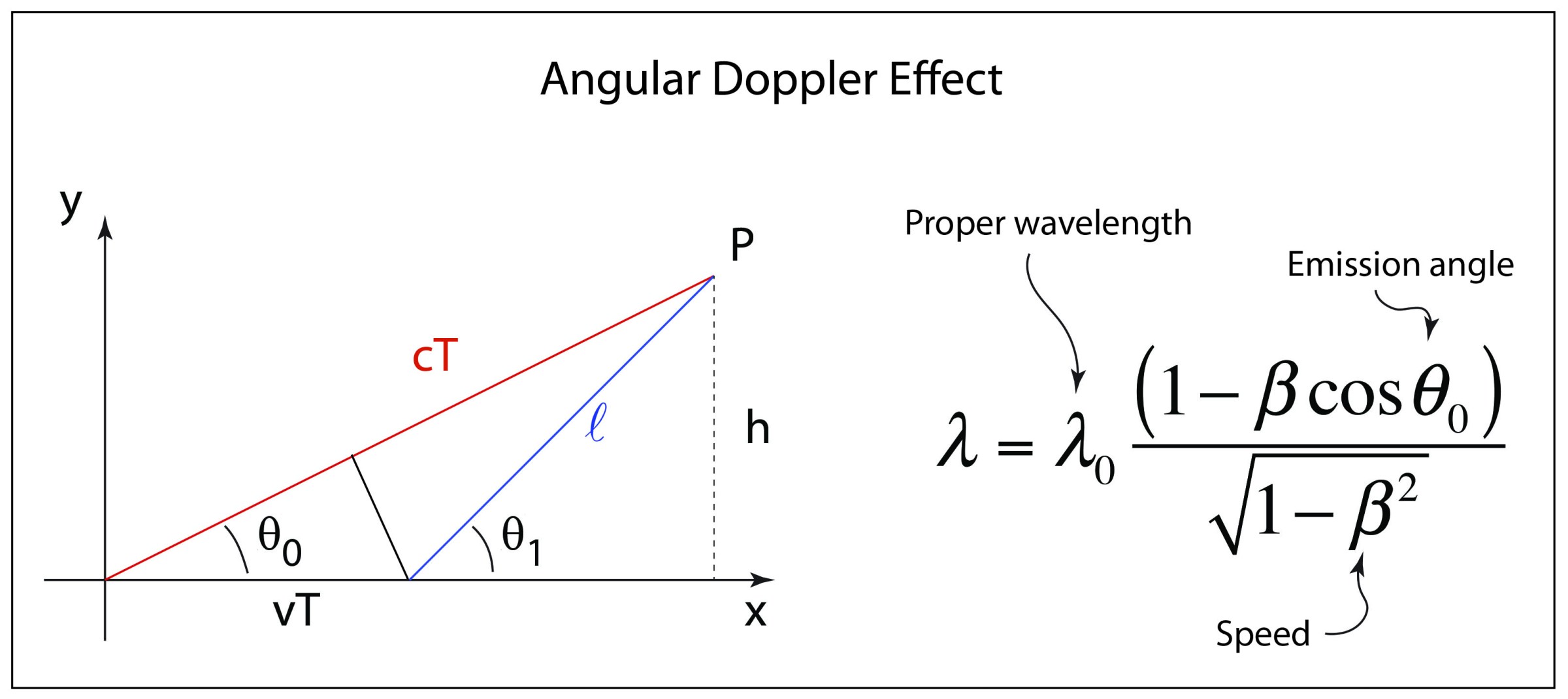
Source: Galileo unbound blog
The relativistically-correct Doppler effect equation is:
$$ \lambda = \lambda_{0} \frac{1 - \beta \cos \theta_{0}}{\sqrt{ 1 - \beta^2 }} = \lambda_{0} \gamma(1 - \beta \cos \theta_{0}) $$
Where $\theta_0$ is the angle measured in the frame of the light emitter from its origin with respect to the point $P$, $\lambda_0$ is the proper wavelength (the wavelength in the light emitter’s frame), and $\lambda$ is the wavelength measured by the observer at $P$. Note that the equivalent formula in terms of frequency $f$ is given by:
$$ f = f_{0} \frac{\sqrt{ 1 - \beta^2 }}{1 - \beta \cos \theta_{0}} = \frac{f_{0}}{\gamma(1 - \beta \cos \theta_{0})} $$
The result is that light emitted by a source moving away from an observer becomes redshifted (longer wavelength, shorter frequency) while light emitted by a source moving towards an observer becomes blueshifted (shorter wavelength, higher frequency). This is significant in astronomical observations of particle jets moving close to the speed of light.
The action principle and the Lagrangian formulation
Before we continue further, it is useful to give a brief description of Lagrangian mechanics, since it will be used a lot when we discuss motion in general relativity. The action principle says that everything in the universe has a special quantity known as the action $S$, which takes the form:
$$ S[\mathbf{r}, \dot{\mathbf{r}}, t] = \int \mathcal{L}(\mathbf{r}, \dot{\mathbf{r}}, t) dt, \quad \mathcal{L} = K - U $$
Where $\mathcal{L}$ is known as the Lagrangian, and (classically) is the difference between an object’s kinetic energy $K$ and potential energy $U$. In the case of a (Newtonian) free particle, we can set $U = 0$, giving us:
$$ \mathcal{L} = \frac{1}{2} mv^2 $$
Of course, this is not relativistically-correct, but is a good approximation for low velocities. The equations of motion can be obtained by the calculus of variations, which says that the path $x^i(t)$ travelled by a particle with Lagrangian $\mathcal{L}$ is given by the Euler-Lagrange equation:
$$ \frac{d}{dt}\left( \frac{\partial \mathcal{L}}{\partial \dot{x}^{i} } \right) = \frac{\partial \mathcal{L}}{\partial x^{i} } $$
Where $x^i$ is the three-position of an object, and $\dot x^i = \frac{dx^i}{dt}$ is its three-velocity. Note that the Euler-Lagrange equation is actually a system of differential equations, with one for each component of $x^i$. For instance, in three dimensions and in Cartesian coordinates, we have three Euler-Lagrange equations:
$$ \begin{align*} \frac{d}{dt}\left( \frac{\partial \mathcal{L}}{\partial \dot{x} } \right) = \frac{\partial \mathcal{L}}{\partial x } \\\frac{d}{dt}\left( \frac{\partial \mathcal{L}}{\partial \dot{y} } \right) = \frac{\partial \mathcal{L}}{\partial y } \\ \frac{d}{dt}\left( \frac{\partial \mathcal{L}}{\partial \dot{z} } \right) = \frac{\partial \mathcal{L}}{\partial z } \end{align*} $$
In special relativity, we must replace $dt$ with $d\tau$, and the Lagrangian of a free particle (where $U = 0$) is given by:
$$ S = \int mc^2 d\tau = mc \int \sqrt{ -ds^2 } = mc^2 \int \frac{dt}{\gamma(v)} $$
Which comes from the fact that $ds^2 = -c^2 d\tau^2$ and $dt = \gamma d\tau$, as we have seen previously. The Lagrangian is thus:
$$ \mathcal{L} = \frac{mc^2}{\gamma(v)} $$
This Lagrangian is only dependent on the velocity of the particle, so $\frac{\partial \mathcal{L}}{\partial x^i} = 0$. Meanwhile:
$$ \frac{\partial \mathcal{L}}{\partial \dot{x}^i} = mc^2 \frac{\partial}{\partial \dot{x}^i} \left( \frac{1}{\gamma(v)} \right) $$
Since $\gamma(v) = \dfrac{1}{\sqrt{1 - \beta^2}} = \dfrac{1}{\sqrt{1 - (\dot x^i / c)^2}}$, upon differentiation, we have:
$$ \frac{\partial}{\partial \dot{x}^i} \left( \frac{1}{\gamma(v)} \right) = \frac{1}{2\sqrt{ 1 - (\dot{x}^i / c)^2 }} \cdot \frac{2 \dot{x}^i}{c} = \frac{\gamma \dot{x}^i}{c} $$
Substituting into the Euler-Lagrange equation, we have:
$$ \frac{d}{dt}(\gamma m \dot{x}^i) = 0 $$
This may be written in a more familiar form if we use standard vector notation, giving us:
$$ \frac{d}{dt}(\gamma m \mathbf{v}) = 0 $$
Where we see $\gamma m \mathbf{v}$ is just the relativistic 3-momentum! Note that in the limit of small velocities, $\gamma \approx 1$, so the above reduces to:
$$ \frac{d}{dt}(m \mathbf{v}) = m \mathbf{a} = 0 $$
Which is simply Newton’s second law for a free particle, as we would expect.
Note: For a much more gentle introduction to Lagrangian mechanics, please see the guide to Lagrangian and Hamiltonian mechanics.
The equivalence principle
A key result that led to the development of general relativity is a peculiar fact of the Universe. We observe that gravity is indistinguishable from an accelerating reference frame. For instance, imagine you were in a rocket in interstellar space, far away from all other objects. The rocket is accelerating upwards (along $z$) with constant acceleration $g$, where $g = \pu{9.81 m/s^2}$ is the standard gravitational acceleration of the Earth. You would then feel a “force” pushing you down, although strictly speaking this is not a force; it is the effect of being in an accelerating reference frame (i.e. the accelerating rocket). Mathematically, your acceleration would be $\vec a = -g \hat{z}$.
Now, imagine that your clone is on another rocket, except this time, the rocket on Earth. Your clone would still feel an acceleration of $g$ downwards, because it is on Earth; that is, their acceleration is also $\vec a = -g \hat z$. Imagine both you and your clone are in a completely isolated rocket, with no windows and no other way to see the outside world. Could you or your clone tell which rocket they were in, if they were mysteriously teleported to one of the two rockets? No! They would experience exactly the same acceleration in either rocket, so there is no way they can tell!
![[equivalence-principle.excalidraw.svg|400]]
The mathematical reason why is that gravity acts on all masses equivalently. Recall that the gravitational force from a mass $M$ on another mass $m$ takes the form:
$$ \mathbf{F} = G Mm\left( \frac{\mathbf{r}_{1} - \mathbf{r}_{2}}{|\mathbf{r}_{1} - \mathbf{r}_{2}|^3} \right) $$
Meanwhile, Newton’s second law tells us that:
$$ \mathbf{F} = m \mathbf{a} $$
Thus, equating the two expressions, we have:
$$ \begin{gather*} m \mathbf{a} = G Mm\left( \frac{\mathbf{r}_{1} - \mathbf{r}_{2}}{|\mathbf{r}_{1} - \mathbf{r}_{2}|^3} \right) \\ \Rightarrow \,\mathbf{a} = GM \left( \frac{\mathbf{r}_{1} - \mathbf{r}_{2}}{|\mathbf{r}_{1} - \mathbf{r}_{2}|^3} \right) \end{gather*} $$
Notice that the gravitational acceleration of the mass $m$ does not depend on its own mass! Neglecting air resistance, this is why a feather and a hammer fall at the same speed in a gravitational field, despite their very different masses (famously demonstrated by astronaut David Scott on the moon; see this YouTube video). The ideas we have presented are backed by more than a century of experiments, and are together known as the equivalence principle. There are actually two formulations of the equivalence principle:
- The weak equivalence principle says that in any gravitational field, a particle in freefall (i.e. without any non-gravitational forces) has the same acceleration regardless of its mass
- The strong equivalence principle says that it is impossible to perform any experiment that could distinguish between an accelerating reference frame and a gravitational field
The equivalence principle is the fundamental basis of general relativity and pretty much the entire theory is based on it. It is also very useful in performing approximate calculations without needing to use the full Einstein field equations (more on that later). We'll look at three examples: gravitational redshift, gravitational time dilation, and gravitational bending of light.
Gravitational redshift
When light travels out of a gravitational field, we find that it becomes redshifted (increases in wavelength). This is known as gravitational redshift, which can be derived directly from the equivalence principle.
Consider a rocket travelling through space with uniform acceleration $\mathbf{a} = a \hat y$. A light pulse is emitted at the bottom of the rocket and travels upwards, reaching the top of the rocket after a certain time interval $\Delta t$. We know that light travels at the constant speed of $c$, which is independent of the reference frame. However, the top of the rocket (like the rest of the rocket) is accelerating upwards, meaning that in the same time interval, the top of the rocket has increased in velocity by $v = a \Delta t$. As we saw earlier, the Doppler shift formula is given by:
$$ f = f_0 \left(1 + \frac{v}{c}\right) $$
Where $f_0$ is the original frequency of the light, $f$ is its Doppler-shifted frequency, and $v$ is the velocity of the moving reference frame (in this case, the rocket). We know that $v = a \Delta t$, and since light travels at a constant velocity $c$, we have $h = c \Delta t$, so $\Delta t = h/c$. Combining the two together, we get $v = a h/c$, so if we substitute this in for $v$ we get:
$$ f = f_0 \left(1 + \frac{a h}{c^2}\right) $$
Therefore, the (Doppler-shifted) frequency $f$ by the time it reaches the top of the rocket is related to its original frequency by:
$$ \frac{f}{f_0} = 1 + \frac{ah}{c^2} $$
So far, there is nothing particularly gravitational about this formula; it would hold for any accelerating reference frame. But since we know from the equivalence principle that an accelerating reference frame is indistinguishable from gravity. This means that we can just substitute in $\mathbf{a} = -g \hat y$ for the gravitational field of the Earth, giving us:
$$ \frac{f}{f_0} = 1 - \frac{gh}{c^2} $$
Note that $f/f_0 = \lambda_0/\lambda$ in terms of wavelength, so we can equivalently write this as:
$$ \frac{\lambda_0}{\lambda} = 1 - \frac{gh}{c^2} $$
We can also write this equivalently in terms of the dimensionless Doppler shift factor $z$, as follows:
$$ z \equiv \frac{\lambda}{\lambda_{0}} -1 = \frac{\Delta \lambda}{\lambda_{0}} = \frac{gh}{c^2} $$
Note: It may also be useful to know that the Doppler shift factor $z$ can be expressed in terms of frequency as $z = \frac{f_0 - f}{f} = -\Delta f/f$, where $\Delta f = f - f_0$.
Where $\Delta \lambda = \lambda - \lambda_{0}$ is the change in the wavelength due to gravitational redshift, assuming a constant gravitational field. We identify $gh = |\Phi|$ as an approximation for the (Newtonian) gravitational potential near the surface of the Earth, so we can generalize the above formula to:
$$ \frac{\Delta \lambda}{\lambda_{0}} = \frac{|\Phi(R)|}{c^2} = \frac{GM}{c^2 R}, \quad \Phi(r) = -\frac{GM}{r} $$
Where $R$ is the distance from the center of the gravitating body (for instance, the Earth) to the light receiver and $M$ is its mass. This formula is valid with respect to a receiver located infinitely-far away, since $\Phi(\infty) = 0$, meaning that gravity (and therefore gravitational redshift) vanishes at infinity. But if we want to compare two observers at known distances $r_1, r_2$ from the center of the gravitating body, where $r_1 > r_2$, then the more precise formula would be:
$$ \begin{align*} \frac{\Delta \lambda}{\lambda_{0}} &= \frac{\Phi(r_{1}) - \Phi(r_{2})}{c^2} \\ &= \frac{GM}{c^2}\left( \frac{1}{r_{2}} - \frac{1}{r_{1}} \right), \quad r_{1} > r_{2} \end{align*} $$
Where we can see that in the limit $r_1 \to \infty$, and with $r_2 = R$ (for an observer on the surface of the Earth), this reduces to $\Delta \lambda/\lambda_0 = GM/(c^2 R)$. Alternatively, expressed in terms of frequency, we have:
$$ \begin{align*} \frac{\Delta f}{f} &= \frac{\Phi(r_{1}) - \Phi(r_{2})}{c^2} \\ &= \frac{GM}{c^2} \left( \frac{1}{r_{2}} - \frac{1}{r_{1}} \right), \quad r_{1} > r_{2} \end{align*} $$
The effects of gravitational redshift are very small, but it can be detected using sensitive instruments: most famously in the Pound-Rebka experiment in the 1950s. The effects are far more substantial in strong gravitational fields, such as around white dwarfs and neutron stars.
Note: Gravitational redshift occurs because light is travelling out of a gravity well and losing energy; lower energy light has a longer wavelength by the time it reaches a receiver. But if light is travelling into a gravity well, it actually gains energy. This is known as gravitational blueshift and it results in light that has a shorter wavelength at the receiver compared to the emitter.
Summary for gravitational redshift
The following formulas and tables are suitable for both calculating gravitational blueshift (when light travels into a gravity well) and gravitational redshift (when light travels out of a gravity well). In below formulae, assume that location $A$ is higher up in a gravity well compared to location $B$. For instance, $A$ could be on a satellite/spacecraft and $B$ could be on the surface of the Earth.
| Variable | Definition |
|---|---|
| $r_A$ | Position of location $A$ from the center of the gravitating body (e.g. from the center of the Earth). Note that $r_A > r_B$. |
| $r_B$ | Position of location $B$ from the center of the gravitating body (e.g. from the center of the Earth). Note that $r_A > r_B$. |
| $\lambda_A$ | Wavelength measured at $A$ |
| $\lambda_{B}$ | Wavelength measured at $B$ |
| $f_A$ | Frequency measured at $A$ |
| $f_{B}$ | Frequency measured at $B$ |
| $\Delta \lambda = \lambda_{B} - \lambda_A$ | Change in wavelength between $A$ and $B$ |
| $\Delta f = f_{B} - f_A$ | Change in frequency between $A$ and $B$ |
| $\Phi(\mathbf{r}) = -\frac{GM}{r}$ | Gravitational potential |
| $\Delta \Phi = \Phi(r_{A}) - \Phi(r_{B})$ | Difference in gravitational potential between $A$ and $B$; $\Delta \Phi$ is always positive |
| $z$ | Doppler shift factor; $z = \Delta \lambda/\lambda_A = -\Delta f/f_{B}$ |
A qualitative summary of the effects of gravitational redshift/blueshift is given below:
| Scenario | Effect | Doppler shift | Wavelength | Frequency |
|---|---|---|---|---|
| Light travelling $A \to B$ | Blueshift | $z < 0$ | $\Delta \lambda < 0$ | $\Delta f > 0$ |
| Light travelling $B \to A$ | Redshift | $z > 0$ | $\Delta \lambda > 0$ | $\Delta f < 0$ |
Assuming $r_A > r_B$, the formulas for the change in wavelength and change in frequency, respectively, are:
$$ \begin{align*} \frac{\Delta \lambda}{\lambda_A} &= \frac{GM}{c^2}\left( \frac{1}{r_B} - \frac{1}{r_A} \right) \\ \frac{\lambda_B}{\Delta \lambda} &= 1 + \left[ \frac{GM}{c^2}\left( \frac{1}{r_B} - \frac{1}{r_A} \right) \right]^{-1} \\ \frac{\Delta f}{f_{B}} &= \frac{GM}{c^2} \left( \frac{1}{r_B} - \frac{1}{r_A} \right) \\ \frac{f_A}{\Delta f} &= \left[ \frac{GM}{c^2}\left( \frac{1}{r_B} - \frac{1}{r_A} \right) \right]^{-1} - 1 \end{align*} $$
Note: The interactive calculator here can be used to compute actual values of blueshift/redshift in different scenarios.
Gravitational time dilation
Consider two clocks in a gravitational field, separated by a vertical distance $h$. To make this scenario more concrete, let’s say that one clock is located on a GPS satellite (which carry atomic clocks) and one clock is located on the surface of the Earth. A light ray is sent from the ground and arrives at the satellite at some time later. What time does the satellite’s clock measure?
Here, we won’t do the full derivation, but the equivalence principle allows us to switch to an accelerating frame, perform the calculations, and simply make the replacements $\mathbf{a} = -g\hat y$ and $gh = \Phi$. to generalize the result to gravitational fields. The end result is:
$$ \tau_{1} = \left( 1 + \frac{\Phi_{1} - \Phi_{2}}{c^2} \right)\tau_{2} $$
Or in terms of differentials:
$$ d\tau_{1} = \left( 1 + \frac{\Phi_{1} - \Phi_{2}}{c^2} \right)d\tau_{2} $$
Where $(\Phi_1 - \Phi_2)$ is always positive (so $\tau_1 \geq \tau_2$) and:
- $\tau_1$ is the time elapsed on the satellite (or in general, for any distant observer)
- $\tau_2$ is the time elapsed on the ground (or in general, for any observer closer to the gravitating body)
- $\Phi_1$ is the gravitational potential at the satellite (or in general, for any distant observer)
- $\Phi_2$ is the gravitational potential at the ground (or in general, for any observer closer to the gravitating body)
If we integrate both sides, we obtain:
$$ \Delta \tau_{1} = \left( 1 + \frac{\Delta \Phi}{c^2} \right) \Delta \tau_{2} $$
Where once again, $\Delta \Phi$ is always positive, meaning that the time elapsed on the satellite will always be greater than that elapsed on the Earth. That is to say, clocks tick slower in a gravitational field. This has an interesting consequence in that it allows for the possibility of gravitational time travel. In principle, it is possible to send a person very close to an astronomical body with an extremely strong gravitational field (e.g. a black hole) and then return them to Earth (ignoring that obviously we cannot do this with today’s technology). The person would then have travelled forward in time, since less time would’ve elapsed for them as compared to a distance observer on Earth.
Show table of contents Back to all notes