In-Depth Quantum Mechanics, Part III
This page is print-friendly. Simply press Ctrl + P (or Command + P if you use a Mac) to print the page and download it as a PDF. Report an issue or error here.
Table of contents
Note: it is highly recommended to navigate by clicking links in the table of contents! It means you can use the back button in your browser to go back to any section you were reading, so you can jump back and forth between sections!
In this third installment of the quantum mechanics series, we'll build on what we learned in the previous two parts to gain a deep understanding of quantum theory and how to apply it to solve real-world problems. We'll cover a variety of approximation techniques to analyze systems too complex to find an exact solution, and use these techniques to solve some of the most famous problems in quantum mechanics.
Chapter guide for Quantum Mechanics
- Part 1 covers the basic ideas of quantum mechanics and its fundamental formalism.
- Part 2 covers applications of quantum mechanics as well as more advanced quantum-mechanical systems.
- Part 3 covers approximation methods in quantum mechanics, as well as applications to a variety of systems. You are reading this part right now.
- Part 4 covers advanced topics in quantum mechanics, including relativistic quantum mechanics, second quantization, and quantum field theory.
Stationary perturbation theory
Perturbation theory exists when we come upon a problem that is too complicated to solve exactly. These problems are often (but not always) variations of existing problems. For instance, we know the solution of the hydrogen atom, since that can be solved exactly, but it turns out that for the helium atom, which has just one more electron than the hydrogen atom, there is no analytical solution! In such cases, we typically resort to one of two options:
- Solve the system on a computer using numerical methods
- Find an approximate analytical solution
The second option is what we'll focus on here, since numerical methods in quantum mechanics is a topic broad enough for an entire textbook on its own. This approach - making calculations using approximations - is known as perturbation theory, and it allows us to solve many kinds of problems that cannot be solved exactly.
Note: Perturbation theory, despite its association with quantum mechanics, is actually a far more general technique for solving complicated differential equations (even those describing classical systems). For more information, see this excellent article on a classical application of perturbation theory.
First off, we should mention that there are two general kinds of perturbation theory in quantum mechanics: stationary perturbation theory, which (as the name suggests) applies only for stationary (time-independent) problems, and time-dependent perturbation theory, which applies for problems that explicitly depend on time. Right now, we'll be focusing on stationary perturbation theory; we'll get to the time-dependent version later. While there are notable differences, both types of perturbation theory use the same general method: a complicated system is approximated as a simpler, more familiar system with some added corrections (called perturbations). By computing these correction terms, we are then able to find an approximate solution to the system, even if there is no exact analytical solution.

A description of perturbation theory from XKCD.
Non-degenerate perturbation theory
We will first review the simplest type of stationary perturbation theory, known as non-degenerate perturbation theory (also known as Rayleigh-Schrödinger perturbation theory), which applies to quantum systems without degeneracy (meaning that each eigenstate is uniquely associated with a distinct energy eigenvalue of the Hamiltonian). It turns out that this is in many cases an overly simplified assumption, but the methods we will develop here will be extremely useful for our later discussion of degenerate perturbation theory that accurately describes a variety of real-world quantum systems.
Mathematically-speaking, non-degenerate perturbation theory assumes that the Hamiltonian of a complicated system can be written as a sum of a Hamiltonian $\hat H_0$ with an exact solution and a small perturbation $\Delta \hat{H}$, such that:
$$ \hat{H} = \hat{H}_{0} + \Delta \hat{H}, \quad \Delta \hat{H} = \lambda\hat{W} $$
Here $\hat H_0$ is known as the unperturbed Hamiltonian or free Hamiltonian. For instance, $\hat H_0$ might be the Hamiltonian of a free particle, or of the hydrogen atom, or the quantum harmonic oscillator. The key commonality here is that $\hat H_0$ must be the Hamiltonian of a simpler system that can be analytically solved.
Note: It is common to write $\Delta \hat{H}$ without the operator hat, and it is also common to denote it as $V$ (confusingly). Be aware that in all cases, $W$ is an operator, not a function!
On top of $\hat H_0$ we add the perturbation $\Delta \hat{H}$, which represents the deviations (also called perturbations) of the system's Hamiltonian as compared to the simpler system. This perturbation is assumed to be small, so we scale it by a small number $\lambda$ (where $\lambda \ll 1$), giving us a term of $\Delta \hat{H} = \lambda \hat W$ where $\hat W$ is some arbitrary operator representing perturbations to the Hamiltonian. If we write out the Schrödinger equation for the system, we have:
$$ \hat{H}|\varphi_{n}\rangle = E_{n} |\varphi_{n}\rangle \quad \Rightarrow \quad (\hat{H}_{0} + \lambda\hat{W})\varphi_{n}\rangle = E_{n} |\varphi_{n}\rangle $$
Note that when we take the limit $\lambda \to 0$, the perturbation vanishes, and the Hamiltonian is exactly the unperturbed Hamiltonian $\hat H_0$. This is why perturbation theory is an approximation; it assumes that the simpler system's Hamiltonian $\hat H_{0}$ is already close enough to the more complicate system's Hamiltonian $\hat H$ that $\hat H_0$ can be used to approximate $\hat H$.
The key idea of perturbation theory is that we assume a series solution for $\hat{H}|\varphi_{n}\rangle = E_{n}|\varphi_{n}\rangle$. More accurately, we assume that we can write the solution in terms of a power series in powers of $\lambda$. Now, this assumption doesn't always work - in fact there are some systems where it doesn't work at all - but using this assumption makes it possible to find an approximate solution using analytical methods, which is "good enough" for most purposes. Remember, in the real world, it is impossible to measure anything to infinite precision, so having an approximate answer to a problem that is close enough to the exact solution is often more than sufficient to make testable predictions that align closely with experimental data.
Derivation of non-degenerate perturbation theory
To begin, remember that we aim to find the approximate wavefunctions and eigenenergies of the Hamiltonian. We also assume that the exact eigenstates $|\psi\rangle$ can be expressed as a power series in $\lambda$:
$$ \begin{align*} |\varphi_{n}\rangle &= \sum_{m = 0}^\infty \lambda^m|\varphi_{n}^{(m)}\rangle \\ &=|\varphi_{n}^{(0)}\rangle + \lambda|\varphi_{n}^{(1)}\rangle + \lambda^2|\varphi_{n}^{(2)}\rangle + \dots \end{align*} $$
Here, remember that $|\varphi_{n}\rangle$ is the exact solution to the system (representing all $n$ exact eigenstates of the complicated Hamiltonian $\hat H$), but $|\varphi_{n}^{(0)}\rangle, |\varphi_{n}^{(1)}\rangle, |\varphi_{n}^{(2)}\rangle, \dots$ are successive states whose sum converges to the exact eigenstates of the system. (For those who need a refreshed on power series please see the series and sequences guide). Be aware that the brackets $(1), (2), \dots$ are not exponents; rather they are labels for the successive sets of eigenstates (the first set of eigenstates, the second, the third, and so forth). By summing up infinitely many of these terms in the expansion of the Hamiltonian's eigenstates, we would in principle get the exact eigenstates of the complicated Hamiltonian.
In the same way, we assume that the system's energy eigenvalues $E_n$ can also be written as a power series in $\lambda$, given by:
$$ \begin{align*} E_{n} &= \sum_{m=0}^\infty \lambda^m E_{n}^{(m)} \\ &= E_{n}^{(0)} + \lambda E_{n}^{(1)} + \lambda^2 E_{{n}}^{(2)} + \dots \end{align*} $$
The first term in the expansion, $E_n^{(0)}$, as we'll see, are simply the energy eigenvalues of the unperturbed Hamiltonian $\hat H_0$. The subsequent terms $E_{n}^{(1)}$, $E_{n}^{(2)}$ are known as the first-order correction and second-order correction to the energy eigenvalues, since they respectively have coefficients of $\lambda^1$ and $\lambda^2$. By summing up infinitely many of these terms in the expansion of the energy, we would in principle get the exact energies.
Now, if we substitute our power series solution into the Hamiltonian's eigenvalue equation $\hat{H}|\varphi_{n}\rangle = E_{n}|\varphi_{n}\rangle$, we have:
$$ \begin{align*} (\hat{H}_{0} + \lambda \hat{W})(|\varphi_{n}^{(0)}\rangle &+ \lambda|\varphi_{n}^{(1)}\rangle + \lambda^2|\varphi_{n}^{(2)}\rangle + \dots) \\ &= (E_{n}^{(0)} + \lambda E_{n}^{(1)} + \lambda^2 E_{{n}}^{(2)} + \dots)(|\varphi_{n}^{(0)}\rangle + \lambda|\varphi_{n}^{(1)}\rangle + \lambda^2|\varphi_{n}^{(2)}\rangle + \dots) \end{align*} $$
Distributing the left-hand side gives us:
$$ \begin{align*} \hat{H}_{0}\bigg(|\varphi_{n}^{(0)}\rangle &+ \lambda|\varphi_{n}^{(1)}\rangle + \lambda^2|\varphi_{n}^{(2)}\rangle + \dots\bigg) + \lambda \hat{W}\bigg(|\varphi_{n}^{(0)}\rangle + \lambda|\varphi_{n}^{(1)}\rangle + \lambda^2|\varphi_{n}^{(2)}\rangle + \dots\bigg) \\ &= E_{n}^{(0)}\left(|\varphi_{n}^{(0)}\rangle + \lambda|\varphi_{n}^{(1)}\rangle + \lambda^2|\varphi_{n}^{(2)}\rangle + \dots\right) \\ &\qquad+ \lambda E_{n}^{(1)}\left(|\varphi_{n}^{(0)}\rangle + \lambda|\varphi_{n}^{(1)}\rangle + \lambda^2|\varphi_{n}^{(2)}\rangle + \dots\right)\\ &\qquad+ \lambda^2 E_{n}^{(2)}\left(|\varphi_{n}^{(0)}\rangle + \lambda|\varphi_{n}^{(1)}\rangle + \lambda^2|\varphi_{n}^{(2)}\rangle + \dots\right) \end{align*} $$
If we do some algebraic manipulation to group terms by powers of $\lambda$, we get:
$$ \begin{align*} % LHS of equation \hat{H}_{0}|\varphi_{n}^{(0)}\rangle &+ \lambda \left(\hat{H}_{0}|\varphi_{n}^{(1)}\rangle + \hat{ W}|\varphi_{n}^{(0)}\rangle\right) + \lambda^2\left(\hat{H}_{0}|\varphi_{n}^{(2)}\rangle + \hat{W}|\varphi_{n}^{(1)}\rangle\right) + \dots \\ &= % RHS of equation E_{n}^{(0)}|\varphi_{n}^{(0)}\rangle + \lambda\left(E_{n}^{(0)}|\varphi_{n}^{(1)}\rangle + E_{n}^{(1)}|\varphi_{n}^{(0)}\rangle\right) + \lambda^2 \left(E_{n}^{(0)}|\varphi_{n}^{(2)}\rangle + E_{n}^{(1)}|\varphi_{n}^{(1)}\rangle + E_{n}^{(2)}|\varphi_{n}^{(0)}\rangle\right) + \dots \end{align*} $$
Notice how each term on the left-hand side of the equation now corresponds to a term on the right-hand side with the same power of $\lambda$. Thus, by equating the quantities in the brackets for every power of $\lambda$, we get a system of equations to solve for each order of $\lambda$:
$$ \begin{align*} \mathcal{O}(\lambda^0):& \quad E_{n}^{(0)}|\varphi_{n}^{(0)}\rangle \\ \mathcal{O}(\lambda^1):& \quad \lambda \left(\hat{H}_{0}|\varphi_{n}^{(1)}\rangle + \hat{W}|\varphi_{n}^{(0)}\rangle\right) = \lambda\left(E_{n}^{(0)}|\varphi_{n}^{(1)}\rangle + E_{n}^{(1)}|\varphi_{n}^{(0)}\rangle\right) \\ \mathcal{O}(\lambda^2):& \quad \lambda^2\left(\hat{H}_{0}|\varphi_{n}^{(2)}\rangle + \hat{W}|\varphi_{n}^{(1)}\rangle\right) = \lambda^2 \left(E_{n}^{(0)}|\varphi_{n}^{(2)}\rangle + E_{n}^{(1)}|\varphi_{n}^{(1)}\rangle + E_{n}^{(2)}|\varphi_{n}^{(0)}\rangle\right) \\ & \qquad\vdots \\ \mathcal{O}(\lambda^n): &\quad \lambda^n\left(\hat{H}_{0}|\varphi_{n}^{(n)}\rangle + \hat{W}|\varphi_{n}^{(n-1)}\rangle\right) = \lambda^n\left( E_{n}^{(0)}|\varphi_{n}^{(n)}\rangle + \sum_{j = 1}^n E_{n}^{(j)} \left|\varphi_{n}^{(n - j)}\right\rangle\right) \end{align*} $$
Note: The final, generalized expression for $\mathcal{O}(\lambda^n)$ comes from Dr. Moore's Lecture Notes from Michigan State University.
If we solve every single one of these equations and substituted our found values of the energy corrections $E_n^{(1)}, E_n^{(2)}, E_n^{(3)}, \dots$ and the corrections to the eigenstates $|\varphi_{n}^{(1)}\rangle, |\varphi_{n}^{(2)}\rangle, |\varphi_{n}^{(3)}\rangle, \dots$ we would in principle know the exact eigenstates and energies of the system.
However, in practice, we obviously wouldn't want to solve infinitely many equations, so we usually truncate the series to just a few terms to get an approximate answer to our desired accuracy. For the lowest-order approximation (also called the zeroth-order approximation) we keep only terms of order $\mathcal{O}(\lambda^0)$ - or in simpler terms, drop all terms containing $\lambda$. We are thus left with just the equation for $\mathcal{O}(\lambda^0)$, that is:
$$ \hat H_0|\varphi_n^{(0)}\rangle = E_n^{(0)}|\varphi_n^{(0)}\rangle $$
The result is trivial - this is just the eigenvalue equation of the unperturbed Hamiltonian, which we can solve exactly, and tells us nothing new. However, let's keep going, because the first-order approximation will be where we'll find a crucial result from perturbation theory. In the first-order approximation we include all terms up to first-order in $\lambda$, but no higher-order terms (i.e. ignoring $\lambda^2, \lambda^3, \lambda^4, \dots$ terms). This means that:
$$ |\varphi_{n}\rangle \approx |\varphi_{n}^{(0)}\rangle + \lambda|\varphi_{n}^{(1)}\rangle, \quad E_n \approx E_{n}^{(0)} + \lambda E_{n}^{(1)} $$
We will thus also need to solve the second equation in the system of equations we previously derived, given by:
$$ (\hat{H}_{0} - E_{n}^{(0)})|\varphi_{n}^{(1)}\rangle + \hat{W}|\varphi_{n}^{(0)}\rangle = E_{n}^{(1)}|\varphi_{n}^{(0)}\rangle $$
Now, the trick is to take the inner product of the above equation with the bra $\langle \varphi_n^{(0)}|$. This gives us:
$$ \langle \varphi_n^{(0)}|(\hat{H}_{0} - E_{n}^{(0)})|\varphi_{n}^{(1)}\rangle + \langle \varphi_n^{(0)}|\hat{W}|\varphi_{n}^{(0)}\rangle = \langle \varphi_n^{(0)}|E_{n}^{(1)}|\varphi_{n}^{(0)}\rangle $$
Since $\hat H_0$ is a Hermitian operator, we know that for any two states $|\phi\rangle, |\psi\rangle$, it must be the case that $\langle \phi|\hat H_0|\psi\rangle = \big(\langle \phi|\hat H_0\big)\cdot|\psi\rangle$, meaning that:
$$ \langle \varphi_n^{(0)}|(\hat{H}_{0} - E_{n}^{(0)})|\varphi_{n}^{(1)}\rangle = \underbrace{ \bigg(\langle \varphi_n^{(0)}|\hat{H}_{0} - \langle \varphi_n^{(0)}|E_{n}^{(0)}U\bigg) }_{ \hat H_0|\varphi_n^{(0)}\rangle = E_n^{(0)}|\varphi_n^{(0)}\rangle }|\varphi_{n}^{(1)}\rangle = 0 $$
Thus the entire first term goes to zero, and we are simply left with:
$$ \langle \varphi_n^{(0)}|\hat{W}|\varphi_{n}^{(0)}\rangle = \langle \varphi_n^{(0)}|E_{n}^{(1)}|\varphi_{n}^{(0)}\rangle $$
But since our states are normalized, then it must be the case that the right-hand side reduces to:
$$ \begin{align*} \langle \varphi_n^{(0)}|E_{n}^{(1)}|\varphi_{n}^{(0)}\rangle &= E_{n}^{(1)} \underbrace{ \langle \varphi_n^{(0)}|\varphi_{n}^{(0)}\rangle }_{ 1 } = E_{n}^{(1)} \\ &\Rightarrow~\langle \varphi_n^{(0)}|\hat{W}|\varphi_{n}^{(0)}\rangle = \langle \varphi_n^{(0)}|E_{n}^{(1)}|\varphi_{n}^{(0)}\rangle = E_{n}^{(1)} \end{align*} $$
Finally, after fully simplifying our results, we come to a refreshingly-simple expression for the first-order correction to the eigenenergies:
$$ E_n^{(1)} = \langle \varphi_n^{(0)}|\hat W |\varphi_{n}^{(0)}\rangle $$
Note that the result is very general since it applies for all $n$ eigenstates of the system. Adding in the first-order corrections gives us the (approximate) eigenenergies of the system:
$$ \begin{align*} E_n &\approx E_{n}^{(0)} + \lambda E_{n}^{(1)} \\ &= E_{n}^{(0)} + \lambda \langle \varphi_n^{(0)}|\hat W |\varphi_{n}^{(0)}\rangle \end{align*} $$
Alternatively, if written in terms of the perturbation term $\Delta \hat H$ in the Hamiltonian, we can express the first-order shift in the energy eigenvalues $\Delta E_n^{(1)}$ as:
$$ \Delta E_{n}^{(1)} = \lambda \langle \varphi_n^{(0)}|\hat W |\varphi_{n}^{(0)}\rangle = \langle \varphi_n^{(0)}| \Delta \hat{H} |\varphi_{n}^{(0)}\rangle $$
This is one of the most important equations in all of quantum mechanics and in most cases gives a good approximation to the exact eigenenergies of the system, at least where $\lambda$ is small. It allows us to solve a variety of quantum systems that would otherwise be impossible to solve exactly, and to a large extent, is responsible for why we can perform quantum-mechanical calculations for complicated real-world systems at all!
We can use a similar process to get the first-order correction $|\varphi_n^{(1)}\rangle$ to the eigenstates of the system. We'll spare the derivation for now and just state the results - the first-order correction to the system's eigenstates are given by:
$$ \begin{align*} |\varphi_n^{(1)}\rangle &= \sum_{m\,(m \neq n)} \frac{E_{n}^{(1)}}{\left(\small E_{n}^{(0)} - E_{m}^{(0)}\right)}|\varphi_m^{(0)}\rangle \\ &= \sum_{m\,(m \neq n)} \frac{\langle \varphi_m^{(0)}|\hat W |\varphi_{n}^{(0)}\rangle}{\left(\small E_{n}^{(0)} - E_{m}^{(0)}\right)}|\varphi_m^{(0)}\rangle \end{align*} $$
In most cases, the first-order correction is sufficient to get a "good enough" answer. But we can go further to get a more accurate result! We'll now use a second-order approximation, where we include all terms up to second-order in $\lambda$, but no higher-order terms (i.e. ignoring $\lambda^3, \lambda^4, \lambda^5, \dots$ terms). This means that:
$$ \begin{align*} |\varphi_{n}^{(0)}\rangle &\approx |\varphi_{n}^{(0)}\rangle + \lambda|\varphi_{n}^{(1)}\rangle + \lambda^2|\varphi_{n}^{(2)}\rangle \\ E_{n} &\approx E_{n}^{(0)} + \lambda E_{n}^{(1)} + \lambda^2 E_{{n}}^{(2)} \end{align*} $$
We'll therefore need the third equation in the system of equations we derived at the start of this section, which is given by:
$$ \lambda^2\left(\hat{H}_{0}|\varphi_{n}^{(2)}\rangle + \hat{W}|\varphi_{n}^{(1)}\rangle\right) = \lambda^2 \left(E_{n}^{(0)}|\varphi_{n}^{(2)}\rangle + E_{n}^{(1)}|\varphi_{n}^{(1)}\rangle + E_{n}^{(2)}|\varphi_{n}^{(0)}\rangle\right) $$
Again, making some algebraic simplifications gives us:
$$ (\hat{H}_{0} - E_{n}^{(0)})|\varphi_{n}^{(2)}\rangle + \hat{W}|\varphi_{n}^{(1)}\rangle = E_{n}^{(1)}|\varphi_{n}^{(1)}\rangle + E_{n}^{(2)}|\varphi_{n}^{(0)}\rangle $$
Using our trick from before by taking the inner product with $\langle \varphi_n^{(0)}|$ and exploiting orthogonality, we get:
$$ \underbrace{ \langle \varphi_n^{(0)}|(\hat{H}_{0} - E_{n}^{(0)}) }_{ 0 }|\varphi_{n}^{(2)}\rangle + \langle \varphi_n^{(0)}|\hat{W}|\varphi_{n}^{(1)}\rangle = E_{n}^{(1)}\cancel{ \langle \varphi_n^{(0)}|\varphi_{n}^{(1)}\rangle }^0 + E_{n}^{(2)}\cancel{ \langle \varphi_n^{(0)}|\varphi_{n}^{(0)}\rangle }^1 $$
Where the first term again becomes zero since $\hat{H}_{0}|\varphi_{n}^{(0)}\rangle = E_{n}^{(0)}|\varphi_{n}^{(0)}\rangle$ and since $\hat H_0$ is Hermitian - this follows the same reasoning we explained for the first-order case. We thus have:
$$ E_{n}^{(2)} = \langle \varphi_n^{(0)}|\hat{W}|\varphi_{n}^{(1)}\rangle $$
But we previously found that $|\varphi_n^{(1)}\rangle$ is given by:
$$ |\varphi_n^{(1)}\rangle = \sum_{m\,(m \neq n)} \frac{\langle \varphi_m^{(0)}|\hat W |\varphi_{n}^{(0)}\rangle}{\left(\small E_{n}^{(0)} - E_{m}^{(0)}\right)}|\varphi_m^{(0)}\rangle $$
Thus substituting it into our expression for $E_n^{(2)}$ gives us an explicit expression for the second-order corrections to the eigenenergies of the system:
$$ \begin{align*} E_{n}^{(2)} &= \langle \varphi_n^{(0)}|\hat{W}|\varphi_{n}^{(1)}\rangle \\ &= \langle \varphi_{n}^{(0)}|\hat{W} \left(\sum_{m\,(m \neq n)} \frac{\langle \varphi_m^{(0)}|\hat W |\varphi_{n}^{(0)}\rangle}{\left(\small E_{n}^{(0)} - E_{m}^{(0)}\right)}|\varphi_m^{(0)}\rangle\right) \\ &= \sum_{m\,(m \neq n)} \frac{|\langle \varphi_m^{(0)}|\hat W |\varphi_{n}^{(0)}\rangle|^2}{\left(\small E_{n}^{(0)} - E_{m}^{(0)}\right)} \end{align*} $$
Equivalently, the second-order shift in the energy eigenvalues $\Delta E_n^{(2)}$ is given by:
$$ \Delta E_n^{(2)} = \sum_{m\,(m \neq n)} \frac{|\langle \varphi_m^{(0)}|\Delta\hat H |\varphi_{n}^{(0)}\rangle|^2}{\left(\small E_{n}^{(0)} - E_{m}^{(0)}\right)} $$
While we will not derive it here, one may show that the third-order corrections to the eigenenergies of the system are given by:
$$ E_{n}^{(3)} = \sum_{m~(m \neq n)}\sum_{l} \frac{V_{nl} V_{lm} V_{mn}}{\small (E_{n}^{(0)} - E_{l}^{(0)})(E_{n}^{(0)} - E_{m}^{(0)})} - V_{nn}\sum_{m\,(m \neq n)} \frac{|V_{nm}|^2}{\left(\small E_{n}^{(0)} - E_{m}^{(0)}\right)^2}|\varphi_m^{(0)}\rangle $$
Where here, $V_{ij} \equiv \langle \varphi_{i}^{(0)}|\hat{W}|\varphi_{j}^{(0)}\rangle$. Therefore, the third-order shift in the energy eigenvalues $\Delta E_n^{(3)}$ is:
$$ \Delta E_{n}^{(3)} = \sum_{m~(m \neq n)}\sum_{l} \frac{E_{nl} E_{lm} E_{mn}}{\small (E_{n}^{(0)} - E_{l}^{(0)})(E_{n}^{(0)} - E_{m}^{(0)})} - V_{nn}\sum_{m\,(m \neq n)} \frac{|E_{nm}|^2}{\left(\small E_{n}^{(0)} - E_{m}^{(0)}\right)^2}|\varphi_m^{(0)}\rangle $$
Where $E_{ij} = \langle \varphi_{i}^{(0)}|\Delta\hat{H}|\varphi_{j}^{(0)}\rangle$. Note that in the most general case, we can find the $k$-th order correction to the eigenenergies of the system via:
$$ E_{n}^{(k)} = \langle \varphi_{n}^{(0)}|\hat{W}|\varphi_{n}^{(k - 1)}\rangle $$
Equivalently, the $k$-th order energy shift is given by:
$$ \Delta E_{n}^{(k)} = \langle \varphi_{n}^{(0)}|\Delta \hat{H}|\varphi_{n}^{(k - 1)}\rangle $$
And the exact energies $E_{n}$ of the system are given by the infinite series:
$$ E_{n} = E_{n}^{(0)} + \sum_{m = 1}^\infty \Delta E_{n}^{(m)} $$
In practice, the first few terms of the series are usually enough to yield an exceedingly accurate calculation for the system's energy eigenvalues, and there is no need to calculate beyond the second or third term.
Note: For more in-depth discussion of the formulas for perturbation theory up to arbitrary order, see this Physics StackExchange post.
Example: The ramp in an infinite square well
In our first example of using perturbation theory, let us consider a 1-dimensional infinite square well of length $L$, which has the standard "box" potential:
$$ V_\mathrm{box}(x) = \begin{cases} 0, & 0 \leq x \leq L \\ \infty , & \text{otherwise} \end{cases} $$
The Hamiltonian is therefore:
$$ H = \frac{\hat{p}^2}{2m} + V_\mathrm{box}(x) = \begin{cases} \frac{\hat{p}^2}{2m}, & 0 \leq x \leq L \\ \infty, & \text{otherwise} \end{cases} $$
We have previously calculated energy eigenfunctions and eigenvalues of this potential to be:
$$ \psi_{n}(x) = \sqrt{ \frac{2}{L} } \sin\left( \frac{n \pi x}{L} \right), \quad E_{n} = \frac{n^2 \pi^2 \hbar^2}{2mL^2} $$
Now, let us consider the modified square well with a linear potential term:
$$ H = \frac{p^2}{2m} + V_\mathrm{box} + \alpha x $$
Where $\alpha \ll 1$ is some small constant. We want to find the first-order energy shift caused by this potential (which we may imaginatively call a "ramp potential" since it does look like (and act like) a ramp). Applying the formula for the first-order energy shift, we obtain:
$$ \begin{align*} \Delta E_{n}^{(1)} &= \langle \varphi_n^{(0)}| \Delta \hat{H} |\varphi_{n}^{(0)}\rangle \\ &= \int_{0}^L \psi_{n}(x) \alpha x \psi_{n}(x) dx \\ &= \frac{2 \alpha}{L} \int_{0}^L x \sin^2\left( \frac{n\pi x}{L} \right) dx \\ &= \frac{2\alpha}{L}\left[ \int_{0}^L \frac{x}{2} dx - \cancel{ \int_{0}^L \frac{\cos(2n\pi x / L)}{2}dx }^0\right] \\ &= \frac{\alpha L}{2} \end{align*} $$
Where we applied the identity $\sin^2 x = \frac{1}{2} - \frac{\cos(2x)}{2}$ to split the integral into two simpler integrals. The result tells us that we would observe a first-order energy shift of $\Delta E = \alpha L/2$ upon applying the ramp potential. This makes sense: if the ramp potential is a positive potential (for $\alpha > 0$) the particle is pushed "up" by the ramp and has increased potential energy, while if the ramp potential is a negative potential (for $\alpha < 0$) the particle falls "down" the ramp and has less potential energy.
Example 2: The quantum pendulum
The quantum pendulum is a simple model of a nonlinear harmonic oscillator and a classical problem in perturbation theory. Due to its nonlinearity, it behaves differently from the otherwise-similar quantum harmonic oscillator. The quantum pendulum is described by a Hamiltonian of the form:
$$ \hat{H} = \frac{\hat{L}_{z}^2}{2 m a^2} -\lambda \cos \phi $$
Where $m$ is the mass of the pendulum, while $a$ and $\lambda$ are two constants (with units of length and energy respectively), and it is assumed that $\lambda$ is small such that we can use perturbation theory. The first part of the Hamiltonian is the free Hamiltonian $H_0 = \frac{\hat{L}_{z}^2}{2ma^2}$, which describes a quantum rigid rotor (a rigid rotor is like a spinning top). The Schrödinger equation for the rigid rotor is:
$$ \hat{H}_{0}|\psi_{n}\rangle = \frac{\hat{L}_{z}^2}{2ma^2} |\psi_{n}\rangle = E_{n} |\psi_{n}\rangle $$
It is straightforward to solve for the rigid rotor's eigenstates and energy eigenvalues, since we already know the eigenvalues of $\hat{L}_{z}$, which are simply $n\hbar$ for integer $n$ (we use $n$ instead of the typical $m_l$ for notational clarity). Therefore, the eigenvalues of $\hat L_z^2$ are $n^2\hbar^2$ and:
$$ \frac{\hat{L}_{z}^2}{2ma^2}|\psi_{n}\rangle = \frac{\hbar^2 n^2}{2ma^2}|\psi_{n}\rangle = E |\psi_{n}\rangle $$
From which we can easily "read off" the energy eigenvalues as:
$$ E_{n} = \frac{\hbar^2 n^2}{2ma^2} $$
Meanwhile, the eigenstates can be obtained if we write $L_z^2 = \hbar^2 \frac{\partial^2}{\partial \phi^2}$ in explicit form and solve the eigenvalue equation $L_z^2 \psi = n^2 \hbar^2 \psi$. This gives us eigenfunctions in the form $\psi = A e^{i n \phi}$, upon which the normalization constant can be straightforwardly calculated:
$$ \int_{0}^{2\pi} |\psi(\phi)|^2 d\phi = 2\pi A^2 = 1 \implies A = \frac{1}{\sqrt{ 2\pi }} $$
This gives us the following set of eigenfunctions:
$$ \psi_{n}(\phi) = \frac{e^{in\phi}}{\sqrt{ 2\pi }}, \quad n = 0, 1, 2, 3, \dots $$
First, let's find the first-order correction to the energy eigenvalues, so we will use the first-order perturbation theory formula:
$$ \Delta E_{n}^{(1)} = \langle \varphi_n^{(0)}| \Delta \hat{H} |\varphi_{n}^{(0)}\rangle $$
Here, the perturbation is $\Delta \hat{H} = - \lambda\cos \phi$. Expanding the inner product (which, for our continuous eigenfunctions becomes an integral) therefore gives us:
$$ \Delta E_{n}^{(1)} = -\lambda \int_{0}^{2\pi} \frac{e^{-in\phi}}{\sqrt{ 2\pi }} \cos \phi \frac{e^{in\phi}}{\sqrt{ 2\pi }} d\phi = -\frac{\lambda}{2\pi} \int_{0}^{2\pi} \cos \phi d\phi = 0 $$
We thus find that the first-order correction to the energy eigenvalues are zero. The lack of a first-order correction to the energy, however, doesn't mean the perturbation has no effect. Rather, it suggests that we need to go to second-order. The second-order corrections to the energy eigenvalues are given by:
$$ \Delta E_n^{(2)} = \sum_{m\,(m \neq n)} \frac{|\langle \varphi_m^{(0)}|\Delta\hat H |\varphi_{n}^{(0)}\rangle|^2}{\left(\small E_{n}^{(0)} - E_{m}^{(0)}\right)} $$
Substituting in $\Delta \hat H = -\lambda \cos \phi$ and expanding the inner products, we have:
$$ \begin{align*} \Delta E_{n}^{(2)} &= \sum_{m\,(m \neq n)} \frac{1}{\small E_{n}^{(0)} - E_{m}^{(0)}} \left|(-\lambda)\int_{0}^{2\pi} \psi_{m}(x) \cos \phi \psi_{n}(x) d\phi \right|^2 \\ &= \sum_{m\,(m \neq n)} \frac{\lambda^2}{\small E_{n}^{(0)} - E_{m}^{(0)}} \left| \frac{1}{2\pi} \int_{0}^{2\pi} \cos \phi e^{i(n - m)\phi} d\phi \right|^2 \end{align*} $$
We will now use the following identity:
$$ \frac{1}{\pi}\int_{0}^{2\pi} \cos \phi e^{i(n - m)\phi} d\phi = \delta_{n, 1-m} + \delta_{n, -(1+m)} $$
Where $\delta_{nm}$ is the Kronecker delta, and has a value of zero unless $n = m$ (in which case it equals one). Hence, we have:
$$ \Delta E_{n}^{(2)} = \frac{\lambda^2}{4}\sum_{m\,(m \neq n)} \frac{\left|\delta_{n, 1-m} + \delta_{n, -(1+m)}\right|^2}{\small E_{n}^{(0)} - E_{m}^{(0)}} $$
This allows us to collapse the infinite sum over $m$ because all of its terms are zero except for the cases where $\delta_{n, 1-m}$ and/or $\delta_{n, -(1+m)}$ are nonzero, which occur (respectively) when $n = 1 - m$ and when $n = -(1 + m)$. This gives us three possibilities, where we can rule out one of them easily:
- $n = 1-m$ is individually satisfied.
- $n = -(1 + m)$ is individually satisfied.
- both of the above are satisfied at the same time (this turns out to be impossible because $1 - m = -(1 + m)$ is an equation with no solutions for $m$).
Hence, we need now only examine the first and second possibilities. In the first case, we can rearrange $n = 1-m$ into $m = 1 - n$. Therefore:
$$ E_{n}^{(0)} - E_{m}^{(0)} = E_{n} - E_{1-n} = \frac{\hbar^2 n^2}{2ma^2} - \frac{\hbar^2 (1 - n)^2}{2ma^2} = \frac{\hbar^2}{2ma^2}(2n - 1) $$
In the second case, where $n = -(1 + m)$, we have $n = -1 - m$ hence $m = -1 - n = -(1 + n)$:
$$ E_{n}^{(0)} - E_{m}^{(0)} = E_{n} - E_{-(1 + n)} = \frac{\hbar^2 n^2}{2ma^2} - \frac{\hbar^2 (1 + n)^2}{2ma^2} = -\frac{\hbar^2}{2ma^2}(2n + 1) $$
The formerly infinite sum therefore collapses into two terms (with respective values of $E_{n}^{(0)} - E_{m}^{(0)}$ as given above) giving us:
$$ \begin{align*} \Delta E_{n}^{(2)} &= \frac{\lambda^2}{4} \left( \frac{1}{\hbar^2(2n - 1) / 2 m a^2} - \frac{1}{\hbar^2(2n + 1) / 2 m a^2} \right) \\ &= \frac{ma^2 \lambda^2}{2\hbar^2} \left( \frac{1}{2n-1} - \frac{1}{2n+1} \right) \\ &= \frac{ma^2 \lambda^2}{\hbar^2(4n^2 - 1)} \end{align*} $$
Unlike the first-order correction, the second-order correction is decidedly nonzero. In addition, it is always positive except for the ground state (where it is negative), meaning that it effectively decreases the ground-state energy of the particle and increases the energy of all excited states. This has interesting implications, since a lower (as in more negative) ground state energy generally means that a particle is more tightly bound to a potential. Indeed, an important application of the quantum pendulum model is to describe the Josephson effect in Josephson junctions, a class of superconducting circuits whose operating principle is based on electron tunneling through a gap between two superconductors.
Example 3: The quartic harmonic oscillator
Lastly, we will consider the quartic harmonic oscillator, which is a nonlinear modification of the quantum harmonic oscillator with the following potential:
$$ U_\mathrm{quartic} = \frac{1}{2} m \omega^2 x^2 - \frac{\lambda^4}{4!} x^4 $$
Where $4! = 4 \cdot 3 \cdot 2 \cdot 1 = 24$ and $\lambda$ is a constant that is much smaller than 1. It corresponds to the following Hamiltonian:
$$ \hat{H} = \underbrace{ \frac{\hat{p}^2}{2m} + \frac{1}{2}m \omega^2 x^2 }_{ \hat{H}_{0} } + \underbrace{ \frac{-\lambda}{4!} x^4 }_{ \Delta \hat{H} } $$
This is a toy model frequently used in quantum field theory; in that context, it is known as the quartic theory and is a simple model for interacting particles with no spin (and a precursor to the mathematical description of the Higgs field). It also has an interesting link to our previous example of the quantum pendulum: the quartic potential is effectively (up to some constants) the pendulum potential Taylor-expanded to 4th-order, since:
$$ \Delta \hat{H} = -\lambda \cos \phi = -\lambda + \frac{\lambda}{2!} - \frac{\lambda}{4!} + \dots $$
We want to compute the first-order correction to the energy eigenvalues for the ground state. To start off, the zeroeth-order energy eigenvalues are simply those of the quantum harmonic oscillator:
$$ E_{n}^{(0)} = \left( n + \frac{1}{2} \right)\hbar \omega $$
Hence, the ground state energy (with $n = 0$) is simply:
$$ E_0^{(0)} = \frac{1}{2} \hbar \omega $$
Now, we will compute the first-order energy shift. Recall that the ground state wavefunction of the quantum harmonic oscillator is given by:
$$ \psi_0(x) = \left(\dfrac{m\omega}{\pi \hbar}\right)^{1/4} e^{-m\omega x^2 / (2\hbar)} $$
Therefore, the first-order energy shift is given by:
$$ \begin{align*} \Delta E_{0}^{(1)} &= \langle \psi_{0}^{(0)}|\Delta \hat{H} |\psi_{0}^{(0)}\rangle \\ &= \int_{-\infty}^{\infty} \psi_{0}(x) \frac{-\lambda}{4!} x^4 \psi_{0}(x) dx \\ &= \frac{\lambda}{24} \left( \frac{m\omega}{\pi \hbar} \right)^{1/2} \int_{-\infty}^\infty x^4 e^{-m\omega x^2 / \hbar} dx \end{align*} $$
Now, we make use of the integral identity:
$$ \int_{-\infty}^\infty x^{2n} e^{-ax^2} dx = \sqrt{ \frac{\pi}{a} } \frac{(2n - 1)!!}{(2a)^n} $$
Where $!!$ denotes the double factorial. In our case, letting $n = 2$ and $a = m\omega/\hbar$ we would thus get:
$$ \Delta E_{0}^{(1)} = \frac{\hbar^2 \lambda}{32 m^2 \omega^2} $$
This result is particularly interesting because it is a result that depends on the mass $m$ of the particle. In fact, the ground-state energy shift due to the quartic term is actually inversely-proportional to the mass! This tells us that lighter particles "feel" the quartic potential more strongly, even though the mass of the particle doesn't appear in the quartic potential itself. Additionally, the correction to the ground-state energy is positive, meaning that the particle becomes less tightly bound as a result of the quartic potential. Hence, while a "toy model", the quartic harmonic oscillator is still an important model to study, and even serves as simplified (0+1)-dimensional version of the Higgs mechanism in particle physics.
Non-degenerate perturbation theory works as long as we are dealing with non-degenerate states. Unfortunately, most quantum systems exhibit some amount of degeneracy. The hydrogen atom, for instance, contains $n^2$ or $2n^2$ (depending on whether you count spin) degenerate states for the $n$-th energy level. In the case of $n = 2$ (the first excited state of hydrogen) this means we have 4 (or 8, if you count spin) degenerate states!
The problem with degenerate eigenstates of the Hamiltonian in perturbation theory arises due to the fact that such eigenstates by definition share the same energy. Recall that previously, we noted that the first-order correction to the eigenstates are given by:
$$ |\varphi_n^{(1)}\rangle = \sum_{m\,(m \neq n)} \frac{\langle \varphi_m^{(0)}|\hat W |\varphi_{n}^{(0)}\rangle}{\left(\small E_{n}^{(0)} - E_{m}^{(0)}\right)}|\varphi_m^{(0)}\rangle $$
In degenerate systems, $E_n^{(0)} = E_m^{(0)}$, so we have $E_n^{(0)} - E_m^{(0)} = 0$. This gives us an undefined value of $\frac{1}{0}$. Clearly, this is not a physical solution! Hence, we must turn to degenerate perturbation theory, a version of stationary perturbation theory that specifically applies to degenerate states.
The trick to making degenerate states work in perturbation theory is to perform a change of basis into a new basis. In linear algebra, this process is known as diagonalization. To start with, assume that we have a set of $N$ degenerate eigenstates ${|\varphi_{1}\rangle, |\varphi_{2}\rangle, \dots, |\varphi_{i}\rangle, \dots, |\varphi_{N}\rangle}$. The fact that they are all degenerate is essential here! We now compute the following matrix $H_{ij}$, where:
$$ H_{ij} = \langle \varphi_{i} | \Delta \hat{H} | \varphi_{j} \rangle $$
If we were to write it out explicitly in matrix form, we'd have:
$$ H_{ij} = \begin{pmatrix} \langle \varphi_{1} | \Delta \hat{H} | \varphi_{1} \rangle & \langle \varphi_{1} | \Delta \hat{H} | \varphi_{2} \rangle & \langle \varphi_{1} | \Delta \hat{H} | \varphi_{3} \rangle & \dots & \langle \varphi_{1} | \Delta \hat{H} | \varphi_{N} \rangle \\ \langle \varphi_{2} | \Delta \hat{H} | \varphi_{1} \rangle & \langle \varphi_{2} | \Delta \hat{H} | \varphi_{2} \rangle & \langle \varphi_{2} | \Delta \hat{H} | \varphi_{3} \rangle & \dots & \langle \varphi_{2} | \Delta \hat{H} | \varphi_{N} \rangle \\ \vdots & \vdots & \vdots & \vdots & \vdots \\ \langle \varphi_{i} | \Delta \hat{H} | \varphi_{1} \rangle & \langle \varphi_{i} | \Delta \hat{H} | \varphi_{2} \rangle & \langle \varphi_{i} | \Delta \hat{H} | \varphi_{3} \rangle & \dots & \langle \varphi_{i} | \Delta \hat{H} | \varphi_{N} \rangle \\ \vdots & \vdots & \vdots & \ddots & \vdots \\ \langle \varphi_{N} | \Delta \hat{H} | \varphi_{1} \rangle & \langle \varphi_{N} | \Delta \hat{H} | \varphi_{2} \rangle & \langle \varphi_{N} | \Delta \hat{H} | \varphi_{3} \rangle & \dots & \langle \varphi_{N} | \Delta \hat{H} | \varphi_{N} \rangle \end{pmatrix} $$
While computing all of these inner products may look scary, we often don't need to compute all of them due to orthogonality relations between different states. To find the corrections to the eigenenergies, we must diagonalize this matrix. We can do this by solving the following eigenvalue equation:
$$ \det(H_{ij} - \varepsilon \delta_{ij}) = 0 $$
Where $\delta_{ij}$ is the identity matrix. Our aim is to solve for $\varepsilon$, the eigenvalues of $H_{ij}$. Once we do so, we get a new, diagonalized matrix in the form:
$$ H_{ij}' = \begin{pmatrix} \varepsilon_{1} & & & & & \\ & \varepsilon_{2} & & & & \\ & & \ddots & & & \\ & & & \varepsilon_{i} & & \\ & & & & \ddots & \\ & & & & & \varepsilon_{N - 1} \\ & & & & & & \varepsilon_{N} \end{pmatrix}, \quad H_{ij}' = 0 \text{ if } i \neq j $$
(By definition all the components of $H_{ij}'$ are zero except on the diagonal.) Here, $\varepsilon_i$ is the $i$-th eigenvalue of $H_{ij}$ and there are $N$ eigenvalues total. They physically correspond to the energy eigenvalues of the perturbation $\Delta \hat H$.
Note: while there will always be $N$ eigenvalues, some of these may be repeated eigenvalues or zero. If you see these, don't freak out!
The corresponding eigenvectors of $H_{ij}$ are the basis vectors for the new basis, and are the solutions of the following equation:
$$ (H_{ij} - \varepsilon \delta_{ij}) |\phi\rangle = 0 $$
We therefore now have a set of eigenvalues and a set of eigenvectors at our disposal:
$$ \{\varepsilon_{1}, \varepsilon_{2}, \varepsilon_{3}, \dots, \varepsilon_{N} \}, \quad \{|\phi_{1}\rangle, |\phi_{2}\rangle, |\phi_{3}\rangle, \dots, |\phi_{N}\rangle \} $$
Now is the key part: the energy corrections (shifts) $\Delta E_i$ to the $i$-th eigenstate are exactly equal to the $i$-th eigenvalue of $H_{ij}$! That is, we have:
$$ \Delta E_{i} = \varepsilon_{i} $$
Meanwhile, the corrections to the eigenstates $|\tilde{\varphi}_{i}\rangle$ are:
$$ |\tilde{\varphi}_{i}\rangle = \sum_{j = 1}^N c_{ij} |\varphi_{j}\rangle $$
Where $c_{ij}$ is the $j$-th component of eigenvector $|\phi_i\rangle$. We therefore observe that the new eigenstates have mixed the original degenerate eigenstates into new eigenstates. This "lifts" the degeneracy (a fancy term for essentially saying that the degenerate eigenstates have been made no longer degenerate) and allows the eigenstates of the Hamiltonian to be well-defined, at the cost of requiring the mixing of the original eigenstates.
Applications of stationary perturbation theory
Having solved a few toy models, we now move on to applications of stationary (time-independent) perturbation theory for real quantum systems. We will develop the techniques to analyze complicated systems — and, in the process, go through some of the most famous calculations in the history of quantum mechanics.
The Zeeman effect
We will start with a very famous application of perturbation theory: calculating the energy splitting of an atom within a magnetic field. We observe experimentally that when an atom is subjected to a magnetic field, the wavelengths of light it emits change. Quantum mechanics provides an explanation for why.
To analyze the Zeeman effect, we must go beyond the basic Hamiltonian $\hat H = \dfrac{\hat p^2}{2m} + V(\mathbf{r})$, which has been the staple of all our calculations so far. We need to add a new term to the Hamiltonian that incorporates the effect of the magnetic field, which we denote as $\Delta \hat H_\mathrm{Zeeman}$ and which we call the Zeeman term, leading to the following Hamiltonian:
$$ \hat{H} = \frac{\hat{\mathbf{p}}^2}{2\mu} + V_\mathrm{coulomb}(\mathbf{r}) + \Delta \hat H_\mathrm{Zeeman} $$
Where $\mu$ is the reduced mass. For a uniform magnetic field the Zeeman term $\Delta \hat H_\mathrm{Zeeman}$ is proportional to the magnetic moment operator $\boldsymbol{\mu}_{M}$ and linear in the field, where:
$$ \Delta \hat H_\mathrm{Zeeman} = -\boldsymbol{\mu}_{M} \cdot \mathbf{B}, \quad \boldsymbol{\mu}_{M} = -g\frac{q}{2m_{q}} \hat{\mathbf{L}} $$
Where $\hat{\mathbf{L}}$ is the angular momentum operator, and $g$ is a constant known as the g-factor that describes the ratio between the quantum magnetic dipole moment and the classical magnetic dipole moment. Here, we use $m_q$ to denote the mass of the charged particle we are studying in question (in atoms, the dominant contribution is from electrons, but the nuclei can also play a part in the Zeeman effect). Therefore, the expanded version of the Zeeman term is given by:
$$ \Delta \hat H_\mathrm{Zeeman} = g\frac{q}{2m_{q}} \hat{\mathbf{L}} \cdot \mathbf{B} $$
Up to this point, we have kept our treatment very general and have not assumed a fixed value of the g-factor or the charge of the particle. This is important because an advanced treatment of the Zeeman effect would also take into account the nuclear spin angular momentum, which must take into account (among other things) the different charge and mass of protons compared to electrons. However, in the case of electrons, we have, $m_q = m_e$ (where $m_e$ is the electron mass), and $q = -e$ (where $e$ is the elementary charge constant), giving us:
$$ \Delta \hat H_\mathrm{Zeeman} = -\frac{ge}{2m_{e}} \hat{\mathbf{L}} \cdot \mathbf{B} $$
It is common to express the above in terms of the so-called Bohr magneton $\mu_B$ given by:
$$ \mu_{B} = \frac{e\hbar}{2m_{e}} \approx \pu{9.274 * 10^{−24} J/T} $$
Where $m_e$ is the electron mass. Hence, our rewritten Zeeman Hamiltonian (without taking into account spin) is given by:
$$ \Delta \hat H_\mathrm{Zeeman} = -\frac{g\mu_{B}}{\hbar} \hat{\mathbf{L}} \cdot \mathbf{B} $$
The weak Zeeman effect
If the magnetic field is relatively weak, we may treat the Zeeman term in the Hamiltonian as a perturbation. Therefore, we can use the methods of perturbation theory very straightforwardly. We will first compute the first-order correction with our favorite perturbation theory formula, with our eigenstates being those of the hydrogen atom (that is $|n, \ell, m\rangle$ where we are not including spin yet):
$$ \begin{align*} \Delta E_{n}^{(1)} &= \langle \varphi_n^{(0)}| \Delta \hat{H}_\mathrm{Zeeman} |\varphi_{n}^{(0)}\rangle \\ &= -\frac{g\mu_{B}}{\hbar}\langle n, \ell, m|(\hat{\mathbf{L}} \cdot \mathbf{B}) |n, \ell, m\rangle \end{align*} $$
We will assume a uniform magnetic field $|\mathbf{B}| = B_0 \hat{z}$, hence the component of $\hat{\mathbf{L}}$ that is aligned in the same direction as the field would be $\hat L_z$. As we know eigenvalues of $\hat L_z$ are $m\hbar$, reducing the above to:
$$ \Delta E_{n}^{(1)} = -\frac{g\mu_{B} B_{0}}{\hbar}(m\hbar) \langle n, \ell, m|n, \ell, m\rangle $$
Now, since the eigenstates of the hydrogen atom are normalized (that is, $\langle n, \ell, m|n, \ell, m\rangle = 1$), the bra-ket is simply one, giving us:
$$ \begin{align*} \Delta E_{n}^{(1)} &= -\frac{g\mu_{B} B_{0}}{\hbar}(m\hbar) = -gm \mu_{B}B_{0} \\ n &= 1, 2, \dots, \\ \ell &= 0, 1, 2, \dots, (n-1), \\ m &= -\ell, -(\ell + 1), \dots, (\ell - 1), \ell \end{align*} $$
(Note that $g = 1$ for the weak Zeeman effect as it depends only on orbital angular momentum and not on spin.) Since the energy shift is explicitly dependent on $m$, it is zero for states where $\ell = 0$ and also zero for any states where $m = 0$. However, where $m \neq 0$ the Zeeman effect predicts that the existence of additional energy levels separated by a constant value of $g\mu_B B_0$. These additional energy levels correspond with new eigenstates parametrized by $\ell, m$. The total energy of each state now depends on $n$, $\ell$, and $m$, so instead of $E_n$, we write the energy levels as $E_{n \ell m}$, and they are given by:
$$ \begin{align*} E_{n\ell m} &= E_{n}^{(0)} + \Delta E_{n}^{(1)} \\ &= -\pu{13.6 eV} \cdot \frac{Z^2}{n^2} - m \mu_{B} B_{0} \end{align*} $$
Hence we say that the Zeeman effect lifts the degeneracy of the energy levels, since previously degenerate states have now become non-degenerate. In plainer language, the states that previously shared the same energy now have distinct energies that allow us to easily tell them apart. This will be a continuing theme within our exploration of quantum systems: the application of an external electric or magnetic field lifts the degeneracy of the eigenstates and allows new transitions to become possible (which manifest as new spectral lines within the hydrogen spectrum).
Note: The weak Zeeman effect holds for most "everyday" magnetic fields ($B_0 < \pu{1 T}$). In comparison, Earth's magnetic field has an average strength of $\approx \pu{30-60 \mu T}$, which is 100,000 times weaker. Some exceptions include extremely powerful laboratory magnets and astrophysical magnetic fields (e.g. in stars, pulsars, quasars, etc.), where the weak Zeeman effect is replaced by the strong Zeeman effect.
The anomalous Zeeman effect
It is all well and good using our modified Hamiltonian to describe the Zeeman effect, but if we do out our calculation, we'll find that its predicted energy levels actually deviate a significant amount from experimental values. The discrepancy between experimental observations of Zeeman spectral splitting and our theoretical predictions using our basic formula is known as the anomalous Zeeman effect. An explanation of the anomalous Zeeman effect requires us to consider the effects of electron spin, which we have previously neglected. This means that we must modify the Zeeman term in the Hamiltonian as follows:
$$ \Delta \hat H_\mathrm{Zeeman} \to \frac{q}{2m_{e}}(g_{l}\hat{\mathbf{L}} \cdot \mathbf{B} + g_{s}\hat{\mathbf{L}} \cdot \hat{\mathbf{S}}) $$
Here, $g_l = 1$ and $g_s = 2.0023193$ are the electron orbital g-factor and electron spin g-factor respectively (it is common to simply write $g_s = 2$ as an approximation). The $\hat{\mathbf{L}} \cdot \hat{\mathbf{S}}$ term is known as the LS coupling or spin-orbital coupling term, and comes from the interaction between the electron's spin and the magnetic field of the nucleus in the electron's rest frame. The nucleus is (to a very good approximation) at rest within the atom's rest frame, and hence possesses no magnetic field in that frame; however, in the electron's rest frame the nucleus appears to be moving (an effect of relativity) and hence it has a magnetic field. We will later see LS coupling reappear in the explanation of fine structure, which are tiny corrections to the energy levels of the hydrogen atom that cannot be explained within spin or relativity.
But back to calculating the anomalous Zeeman effect. First, note that it is common to write the Zeeman term in the Hamiltonian (including the spin contribution) in an alternate form as:
$$ \Delta \hat{H}_{Zeeman} = g_{J}\frac{q}{2m_{e}} \hat{\mathbf{J}} \cdot \mathbf{B} $$
Where $\hat{\mathbf{J}} = \hat{\mathbf{L}} + \hat{\mathbf{S}}$ is the total angular momentum operator, $\mu$ is the reduced mass of the atom, and $g_J$ is the Landé g-factor, which is defined as:
$$ \begin{align*} g_{J} &= g_{l} \frac{j(j+1) + \ell(\ell + 1) - s(s+1)}{2j(j+1)} + g_{s} \frac{j(j+1) + s(s+1) - \ell(\ell +1)}{2j(j+1)} \\ &\approx 1 + \frac{j(j+1) + s(s + 1) - \ell(\ell + 1)}{2j(j+1)} \end{align*} $$
Where $\ell$ is the orbital angular momentum quantum number, $s$ is the spin quantum number, $j \equiv \ell + s$ is the total angular momentum quantum number, $g_l = 1$ is the electron orbital g-factor and $g_s = 2.0023193 \dots \approx 2$ is the electron spin g-factor. If you think the formula looks horrible, early 20th-century physicists had it worse: the Landé g-factor was the painstaking result of essentially guess-and-checking based on empirically-observed data. Imagine needing to try essentially every combination of quantum numbers just to get that formula in the end!
However, given that we do know the formula for the g-factor the rest of the derivation is straightforward. Simply apply first-order perturbation theory to the perturbation term $\Delta \hat H_\mathrm{Zeeman}$ (but this time including spin in the hydrogen atom's eigenstates $|n, j, m_{j}, s\rangle$, and recalling that the eigenvalues of $\hat J_z$ are $m_j \hbar$ instead of $m\hbar$), which gives us:
$$ \begin{align*} \Delta E_{n}^{(1)} &= \langle \varphi_n^{(0)}| \Delta \hat{H} |\varphi_{n}^{(0)}\rangle \\ &= -\frac{g_{J}\mu_{B}}{\hbar}\langle n, j, m_{j}, s|(\hat{\mathbf{J}} \cdot \mathbf{B}) |n, j, m_{j}, s\rangle \\ &= -\frac{g\mu_{B} B_{0}}{\hbar}(m_{j}\hbar) = -g_{J}m_{j} \mu_{B}B_{0} \\ n &= 1, 2, \dots, \\ \ell &= 0, 1, 2, \dots, (n-1), \\ s &= \pm \small \frac{1}{2}, \\ j &= 0, \frac{1}{2}, 1, \frac{3}{2}, \dots, \quad |\ell - s\vert \leq j \leq \ell + s, \\ m_{j} &= -j, (-j + 1), \dots, (j - 1), j \end{align*} $$
The vector potential approach
Our derivation so far has followed the approach used by most introductory texts, but it turns out that there is another way to derive the Zeeman effect that is more rigorous. To start, we use the generalized electromagnetic Hamiltonian for a charged particle of mass $m$ and charge $q$ in an electromagnetic field (called the Pauli Hamiltonian, which we'll see again later):
$$ \begin{align*} \hat{H} &= \frac{1}{2m}(\hat{\mathbf{p}} - q \hat{\mathbf{A}})^2 + q\phi \\ &= \frac{1}{2m} \left( \hat{\mathbf{p}}^2 - 2q \hat{\mathbf{p}} \cdot \mathbf{A} + q^2 \mathbf{A}^2 \right) + q\phi \end{align*} $$
Note: Here, $m$ is just the mass of the charged particle, not the magnetic quantum number that we have previously denoted with $m$. We have also ignored spin here for simplicity; we'll see the more generalized treatment with spin later.
Where $\phi$ is the electric scalar potential and $\mathbf{A}$ is the magnetic vector potential (read more on this in the electromagnetic theory guide if unfamiliar), and $\mathbf{B} = \nabla \times \mathbf{A}$. For reasons that we'll cover more in-depth later, we may arbitrarily chose $\mathbf{A}$ such that it is given by:
$$ \mathbf{A} = \frac{1}{2} \mathbf{B} \times \mathbf{r} = \begin{pmatrix} -By \\ Bx \\ 0 \end{pmatrix}, \quad B = \|\mathbf{B}\| $$
Note: If you don't want to wait for the explanation, this is due to a phenomenon called gauge freedom. Specifically, we choose the symmetric gauge by imposing the aforementioned gauge condition $\mathbf{A} = \frac{1}{2}\mathbf{B} \times \mathbf{r}$, in which $\mathbf{B} = \nabla \times \mathbf{A}$.
By substituting in our vector potential, using $\hat{\mathbf{L}} = \mathbf{r} \times \hat{\mathbf{p}}$, and expanding terms, we obtain:
$$ \hat{H} = \frac{1}{2m} \left\{ \hat{\mathbf{p}}^2 + q\mathbf{B} \cdot \hat{\mathbf{L}} + \frac{q^2}{4} (\mathbf{B}^2 \mathbf{r}^2 - (\mathbf{B} \cdot \mathbf{r})^2) \right\} $$
Where the second term is called the diamagnetic term and the third is the paramagnetic term; each successive term is weaker than the last. If we turn off the magnetic field ($\mathbf{B} = 0$) and use the Coulomb potential $\phi = \dfrac{Q}{4\pi \varepsilon_0 r}$ with $Q = Ze$, we recover the Hamiltonian of the hydrogen atom. However, when $\mathbf{B}$ is nonzero, we observe the splitting of energy levels, which is what we find in the Zeeman effect. Indeed, if we ignore the paramagnetic term we exactly reproduce the weak Zeeman effect Hamiltonian that we have been using previously! (As stated previously, it does not cover the anomalous Zeeman effect since we have ignored spin, but a more detailed derivation would also incorporate effect of spin.)
The strong Zeeman effect
For most cases, our formulas for the Zeeman effect and anomalous Zeeman effect work very well, but they fail in the case of strong magnetic fields. In such cases, the Zeeman term can no longer be treated as a small perturbation to the Hamiltonian, and becomes non-perturbative. Instead, we must treat it on equal footing with the rest of the Hamiltonian terms, giving us a Hamiltonian in the form:
$$ \begin{align*} \hat{H} &= \frac{\hat{\mathbf{p}}^2}{2\mu} + V_\mathrm{Coulomb} + \hat H_\mathrm{Zeeman} + \dots \\ &= \frac{\hat{\mathbf{p}}^2}{2\mu} + V_\mathrm{Coulomb} + g_{J}\frac{q}{2m_{e}} \hat{\mathbf{J}} \cdot \mathbf{B} + \dots \end{align*} $$
Where the terms after the Zeeman Hamiltonian represent terms that are much smaller than the Zeeman term. This will be significant once we get to the calculation of the fine structure of hydrogen, where when the Zeeman energy splitting is comparable to (or greater than) the fine-structure energy splitting, the fine-structure contribution will need to be treated as a perturbation "on top of" the Zeeman effect rather than the other way around. Solving this Hamiltonian to find the energy shifts shall be left as an exercise for the reader.
The Stark effect
If magnetic fields can split energy levels, can an electric field do so too? The answer is yes! This is known as the Stark effect. It is weaker than the Zeeman effect, so we will derive both the first and second-order energy corrections using perturbation theory.
The Stark effect is conceptually extremely similar to the Zeeman effect, except we swap the magnetic field with the electric field. To start, we assume a uniform electric field in the form $\vec{\mathcal{E}} = \mathcal{E}_0 \hat z$, where $\mathcal{E}_0$ is the electric field strength. Note that we call the field direction $z$ as a matter of convention, but the choice is technically arbitrary, because we can always rotate our coordinate system such that the electric field aligns with the $z$ axis. The Hamiltonian for the Stark effect can be expressed via the electric dipole moment operator $\boldsymbol{\mu}_E = q\mathbf{r}$ and the electric field as:
$$ \Delta \hat{H}_\mathrm{Stark} = -\boldsymbol{\mu}_{E} \cdot \vec{\mathcal{E}} = -q\mathbf{r} \cdot \vec{\mathcal{E}} $$
From trigonometry, $\mathbf{r} \cdot \hat z = r \cos \theta$, hence one obtains:
$$ \Delta \hat{H}_\mathrm{Stark} = e \mathcal{E}_0 r \cos \theta $$
Where we have also substituted in $q = -e$ (since the Stark effect affects electrons in an atom). We will now do the calculation of the energy shifts that occur due to the Stark effect.
The linear Stark effect
To start, we will calculate the energy shifts to first-order. This is known as the linear Stark effect as it is linear in the electric field strength ($\Delta E \sim \mathcal{E}_0$).
To first-order, we obtain:
$$ \begin{align*} \Delta E_{n}^{(1)} &= \langle \varphi_n^{(0)}| \Delta \hat{H}_\mathrm{Stark}|\varphi_{n}^{(0)}\rangle \\ &= e \mathcal{E}_0 \langle n, \ell, m|r|n, \ell, m\rangle \end{align*} $$
Now, the hydrogen atom's wavefunctions satisfy:
$$ \langle n, \ell, m|\mathbf{r}|n, \ell, m\rangle = 0 $$
One can find this via direct calculation, but we will give a physical argument for why this must be the case. An electric dipole moment only exists where one has an asymmetrical configuration of charge. For states with $\ell = 0$, the orbitals are spherical and therefore exhibit spherical symmetry, hence there can be no dipole moment. Meanwhile, for states with $\ell \neq 0$, the probability density of the orbitals is symmetric along the $z$ axis. Since the charge density is proportional to the probability density, there is no dipole moment either. It is only in the case of mixed orbitals (that is, superpositions of multiple orbitals) that the electric dipole moment is nonzero, not the standard orbitals!

Probability density (proportional to charge density) of the "pure" hydrogen atomic orbitals. Original author: Henning Schomerus from Lancaster University
Therefore, by direct application of non-degenerate perturbation theory, it would appear that the first-order correction to the energies is also identically zero:
$$ \Delta E_{n}^{(1)} = 0 $$
But not so fast! It would be more accurate to say that the first-order correction to the energies of non-degenerate states is zero. This is because we have not considered the fact that many of the eigenstates of the hydrogen atom are degenerate! We know that non-degenerate perturbation theory fails for degenerate states, hence we must now use degenerate perturbation theory instead (for which, it turns out, that nonzero first-order corrections are indeed present).
Using first-order degenerate perturbation theory
To start, we need to pick a set of states that we are degenerate. In the hydrogen atom, the energy levels (at least without correction terms due to fine/hyperfine structure, which we'll talk about later) are only depend on the principal quantum number $n$. (The Stark effect is not directly affected by spin.) Hence, any set of degenerate states must share the same value of $n$. The converse is almost true; states with the same value of $n$ are generally degenerate, with the exception of $n = 1$.
To make our analysis easier, we will only calculate the energy shifts for the first excited state (which has $n = 2$). We could in principal calculate the Stark shift for any energy level (that is, for any $n$) we choose, but the number of degenerate states grows $\sim n^2$ meaning that e.g. $n = 3$ splits into at least 9 states, $n = 4$ splits into at least 16, and (for sake of example) $n = 20$ splits into at least 400 states! That is way too many to analyze for an elementary treatment so we will start with the simplest case of $n = 2$, though we will give a general formula at the end.
The brute-force way to do degenerate perturbation theory
The first way we can go about solving the problem is what I call the "brute-force" approach. Basically, we proceed as follows:
- Create a list of degenerate states for the $n$-th energy level; this will be our basis ${|\varphi_i\rangle}$
- Calculate the matrix elements $H_{ij} = \langle \varphi_i|\Delta \hat H|\varphi_j\rangle$ one by one
- Calculate the eigenvalues and eigenvectors of $H_{ij}$ to get the perturbed energy levels and perturbed eigenstates
Let's start at the first step. In the $n = 2$ energy level, the possible values of $\ell$ are $\ell = 0, 1$ and the possible values of $m$ are $m = 0, \pm 1$. Hence, the 4 states $|2, \ell, m\rangle$ are respectively:
$$ \{|\varphi_i\rangle\} = \left\{|2, 0, 0\rangle, |2, 1, 0\rangle, |2, 1, 1\rangle, |2, 1, -1\rangle \right\} $$
One can write these more explicitly as:
$$ \begin{align*} |\varphi_{1}\rangle &= |2, 0, 0\rangle \\ |\varphi_{2}\rangle &= |2, 1, 0\rangle \\ |\varphi_{3}\rangle &= |2, 1, 1\rangle \\ |\varphi_{4}\rangle &= |2, 1, -1\rangle \end{align*} $$
Note that the specific ordering here is not important since the basis is orthonormal. For instance, we could've chosen $|\varphi_1\rangle$ to be $|2, 1, 0\rangle$ and $|\varphi_2\rangle$ to be $|2, 1, 1\rangle$. The important thing is to list all the degenerate states for a given energy level and make sure you don't accidentally include non-degenerate states.
Now, we compute the matrix elements $\langle \varphi_i|\Delta \hat H|\varphi_j\rangle$ where $\Delta \hat H$ is the Stark Hamiltonian. This is where things become a bit hairy! After all, if we directly substitute into the matrix we get:
$$ H_{ij} = \begin{pmatrix} \langle \varphi_1|\Delta \hat H|\varphi_1\rangle & \langle \varphi_1|\Delta \hat H|\varphi_2\rangle & \langle \varphi_1|\Delta \hat H|\varphi_3\rangle & \langle \varphi_1|\Delta \hat H|\varphi_4\rangle \\ \langle \varphi_2|\Delta \hat H|\varphi_1\rangle & \langle \varphi_2|\Delta \hat H|\varphi_2\rangle & \langle \varphi_2|\Delta \hat H|\varphi_3\rangle & \langle \varphi_2|\Delta \hat H|\varphi_4\rangle \\ \langle \varphi_3|\Delta \hat H|\varphi_1\rangle & \langle \varphi_3|\Delta \hat H|\varphi_2\rangle & \langle \varphi_3|\Delta \hat H|\varphi_3\rangle & \langle \varphi_3|\Delta \hat H|\varphi_4\rangle \\ \langle \varphi_4|\Delta \hat H|\varphi_1\rangle & \langle \varphi_4|\Delta \hat H|\varphi_2\rangle & \langle \varphi_4|\Delta \hat H|\varphi_3\rangle & \langle \varphi_4|\Delta \hat H|\varphi_4\rangle \end{pmatrix} $$
Now, with some patience and grit computing all of those inner products (each of which is an integral) you will find that the matrix elements are the following:
$$ H_{ij} = -3a_{0} e E_{0} \begin{pmatrix} 0 & 1 & 0 & 0 \\ 1 & 0 & 0 & 0 \\ 0 & 0 & 0 & 0 \\ 0 & 0 & 0 & 0 \end{pmatrix} $$
We now need to find the eigenvalues of this matrix. For starters, we don't actually have to find the eigenvalues of the entire $(4 \times 4)$ matrix, since it is zero except for the top-left "corner". This means we ultimately only need to calculate the eigenvalues of this much simpler matrix:
$$ \begin{pmatrix} 0 & 1 \\ 1 & 0 \end{pmatrix} $$
The eigenvalues are $\pm 1$, which gives the (correct) energy shifts of:
$$ \Delta E_\mathrm{Stark} = \pm 3 a_{0} e E_{0} \quad (n = 2) $$
There is nothing specifically wrong with this approach; it does work. Unfortunately, it involves a lot of integrals to compute, because there are $n^2$ degenerate states for the $n$-th energy levels. We saw that even for the first excited state ($n = 2$) we have to get all the eigenvalues for a $(4 \times 4)$ matrix; the next excited state ($n = 3$) would involve solving for the eigenvalues of a $(9 \times 9)$ matrix! Now, I don't know about you, but I'd rather not compute that many integrals or eigenvalues! Hence, let us turn to another, more clever approach that saves us time and avoids the need to calculate so many matrix elements.
The clever way to do degenerate perturbation theory
The "clever" way to do degenerate perturbation theory is to rule out as many of the matrix elements as possible, until we are left with only the nonzero ones. This is generally a much quicker method and involves less work, but does require some reasoning, hence why I call it the "clever" approach.
This approach relies heavily on the selection rules of atomic transitions, which dictate which transitions are possible and which are not. We can figure out a lot of these ourselves! First of all, we know that an atomic transition between two energy levels $E_2 \to E_1$ corresponds to the release of a photon carried an energy $\Delta E = E_{2} - E_{1}$ equal to the difference between the energy levels. Unlike electrons, photons are spin-1 particles, meaning that they carry $\pm 1 \hbar$ units of angular momentum (the sign depends on their specific spin state). To conserve angular momentum, we therefore require that the initial and final states' orbital angular momentum changes by a factor of $\Delta \ell = 1$ or $\Delta \ell = -1$. That is, we obtain the selection rule $\Delta \ell = \pm 1$.
In addition, we know that the allowable values of $m$ range from zero to $\pm \ell$. By the restriction $\Delta \ell = \pm 1$, this means that the change in $m$ must therefore be zero, 1, or -1. Hence we obtain the selection rule $\Delta m = 0, \pm 1$.
Finally, since electrons are spin-1/2 particles, their spin quantum number is always $s = \frac{1}{2}$. Therefore the spin quantum number cannot change during a transition, so $\Delta s = 0$. (This becomes a bit more complicated once we need to consider nuclear spin, which we'll explore once we talk about hyperfine structure, but we can assume $\Delta s = 0$ to be the case for now.)
Collectively, our selection rules are therefore:
$$ \begin{cases} \Delta \ell = \pm 1 \\ \Delta m = 0, \pm 1 \\ \Delta s = 0 \end{cases} $$
Note: These are known as the electric dipole transition selection rules (or E1 selection rules for short) and are not simply the case for the Stark effect, but for all transitions mediated by an electric field!
These selection rules heavily restrict the types of transitions possible in the Stark effect. In our case, it means that each transition between the $n = 2$ states must involve one state with $\ell = 1$ and one state with $\ell = 0$ to satisfy the first selection rule. Hence, we know that the nonzero matrix elements must have $|\varphi_{1}\rangle = |2, 0, 0\rangle$ as one of the states since it is the only state with $n = 2$ that also has $\ell = 0$. Therefore, we only need to consider matrix elements of the forms $\langle \varphi_1|\Delta \hat H|\varphi_i\rangle$ or $\langle \varphi_i|\Delta \hat H|\varphi_1\rangle$. Indeed, since these are symmetric we actually only need to explicitly calculate one of the two forms (the other matrix element would be equal), leaving us with just 4 matrix elements in total out of the original 16. Quite an improvement!
Now, the second selection rule is less immediately helpful because all transitions to/from $|2, 0, 0\rangle$ for the $n = 2$ states satisfy it. However, the Stark effect Hamiltonian is azimuthally-symmetric. This is clear from the form of the Hamiltonian, which explicitly depends on the $r$ and $\theta$ coordinates, but doesn't depend on the $\phi$ coordinate, hence a rotation about the $z$ axis has no effect on the Hamiltonian. Therefore, the $z$-component of the angular component must be conserved. Since $L_z = m\hbar$, it is clear that if $\Delta L_z = 0$, then $\Delta m = 0$ must be true as well! Therefore, our selection rules become additionally restricted to the following:
$$ \begin{cases} \Delta \ell = \pm 1 \\ \Delta m = 0 \\ \Delta s = 0 \end{cases} $$
There is only one transition involving the $|2, 0, 0\rangle$ state that also satisfies $\Delta m = 0$, and it is the transition between the $|2, 0, 0\rangle$ and $|2,1, 0\rangle$ states. Hence, this is the only matrix element we'll need to calculate! By using this "clever" approach, we have drastically cut down the number of matrix elements we need to calculate! Upon doing the calculation, we have:
$$ \begin{align*} \langle 2, 0, 0|\Delta \hat{H} |2, 1, 0\rangle &= e\mathcal{E}_{0} \langle \varphi_{1}|r \cos \theta|\varphi_{2}\rangle \\ &= e\mathcal{E}_{0} \int_{0}^\infty R_{20}(r)R_{21}(r) r^2 dr \int_{0}^{2\pi} \int_{0}^\pi Y^0_{0}(\theta, \phi)^* Y^0_{1}(\theta, \phi) \cos \theta(\sin \theta d \theta d\phi) \\ &= -3a_{0}e \mathcal{E}_{0} \end{align*} $$
And likewise (due to symmetry):
$$ \langle 2,1, 0|\Delta \hat{H}|2, 0, 0\rangle = \langle 2, 0, 0|\Delta \hat{H} |2, 1, 0\rangle = -3a_{0}e \mathcal{E}_{0} $$
The $H_{ij}$ matrix is therefore zero for all terms except for the $H_{12}$ and $H_{21}$ elements, which correspond to the two above transitions. Therefore, we have:
$$ H_{ij} = -3a_{0} e E_{0} \begin{pmatrix} 0 & 1 & 0 & 0 \\ 1 & 0 & 0 & 0 \\ 0 & 0 & 0 & 0 \\ 0 & 0 & 0 & 0 \end{pmatrix} $$
This is the same matrix that we got earlier, and we've already calculated what its eigenvalues are: they are respectively $\pm 3 a_{0}eE_{0}$, hence the energy shifts due to the linear Stark effect are:
$$ \Delta E_\mathrm{Stark} = \pm 3 a_{0}eE_{0} $$
The resulting (normalized) eigenvectors are:
$$ |\phi_{1}\rangle = \frac{1}{\sqrt{ 2 }} \begin{pmatrix} -1 \\ 1 \end{pmatrix}, \quad |\phi_{1}\rangle = \frac{1}{\sqrt{ 2 }} \begin{pmatrix} 1 \\ 1 \end{pmatrix} $$
(The first corresponds to the eigenvalue of $-3a_0 eE_0$ and the second corresponds to the eigenvalue of $+3 a_0 eE_0$). We can now construct the perturbed eigenstates $|\tilde{\varphi}_{i}\rangle$, which are given by:
$$ |\tilde{\varphi}_{i}\rangle = \sum_{j = 1}^N \phi_{ij} |\varphi_{j}\rangle $$
Here, we have $N = 2$ (technically $N = 4$ but there are only two nonzero eigenvectors) and $\phi_{ij}$ denotes the $j$-th component of the eigenvector $|\phi_i\rangle$, which are (respectively):
$$ \phi_{ij} = \frac{1}{\sqrt{ 2 }} \begin{pmatrix} -1 & 1 \\ 1 & 1 \end{pmatrix} $$
Therefore, the perturbed eigenstates are:
$$ \begin{align*} |\tilde{\varphi}_{1}\rangle &= \frac{1}{\sqrt{ 2 }}(|2, 1, 0\rangle - |2, 0, 0\rangle) \\ |\tilde{\varphi}_{2}\rangle &= \frac{1}{\sqrt{ 2 }}(|2, 0, 0\rangle + |2, 1, 0\rangle) \end{align*} $$
Notice how the Stark effect has given us mixed orbitals. These orbitals, unlike the regular atomic orbitals, have asymmetric probability densities (and therefore asymmetric charge distributions) which gives rise to a nonzero electric dipole moment, resulting in the splitting of the spectral lines!
Summary of degenerate perturbation theory in the Stark effect
In the general case for arbitrary $n$, the linear Stark effect predicts that the $n$-th state will split into $2n - 1$ distinct energy levels. A diagram of (some of) the Stark shifts is shown below:

Source: Wikipedia

The Stark effect has applications in spectroscopy as well as in semiconductor optics. The observations of the spectral lines arising from the Stark effect was also historically important in the development of quantum theory, as it could not be explained by classical physics. For those interested in the history of the Stark effect, this YouTube video and this other YouTube video (both by the excellent channel of Dr. Jorge S. Diaz) for more information regarding the history of the Stark effect.
The quadratic Stark effect
Now, we will go beyond first-order and examine the energy shifts to second-order. This is known as the quadratic Stark effect as it is quadratic in the electric field strength ($\Delta E \sim \mathcal{E}_0^2$). Using second-order perturbation theory, it can be shown that the energy shifts are given by:
$$ \Delta E_{n}^{(2)} = -\frac{1}{2} \sum_{i} \sum_{j} \alpha_{ij} \mathbf{E}_i \mathbf{E}_{j} $$
Where $\mathbf{E}$ is the $i$-th component of the electric field (in our simplified case, $\mathbf{E} = \mathbf{E} = 0$ except for $i = j = 3$, where $\mathbf{E}3 = E_0$ Note that if the material is isotropic (which most materials can be assumed to be), the polarizability tensor $\alpha{ij}$ can be expressed as:
$$ \alpha_{ij} = \alpha \delta_{ij}, \quad \alpha_{0} = 4\pi \varepsilon_{0} a_{0}^3 = \text{const.} $$
Where $\alpha_0$ is known as the static electric polarizability. Hence, the expression for the second-order energy shifts for isotropic materials reduces to:
$$ \Delta E_{n}^{(2)} = -\frac{1}{2} \alpha_{0} E_{0}^2 $$
Unlike the linear Stark effect, the quadratic Stark effect does predict an energy shift for the $n = 1$ state (ground state), albeit a very small energy shift. In fact, it predicts an energy shift for all the energy levels! However, even in an extremely powerful electric field of $E_0 = \pu{10^7 V/cm}$ the quadratic stark shift for the $n = 1$ state is only around $\pu{0.05 meV}$, which is a tiny shift. Hence, the Stark effect is generally dominated by the first-order (linear) contribution rather than the second-order (quadratic) contribution.
The generalized Stark effect
We can use the procedure we performed for the first and second-order energy shifts to come up with energy corrections to any desired order. It is left as a challenge for the reader to derive a generalized formula for the Stark energy shifts for arbitrary $n, \ell, m$ (this is an exercise for the adventurous reader because it is not easy to do!) The general solutions for the first, second, and third-order energy shifts are as follows (from section 3.10.2 of Elementary Molecular Quantum Mechanics 2nd ed.):
$$ \begin{align*} \Delta E^{(1)}_{n} &= -\frac{3}{2} e E_{0} a_{0} n(k_{1} - k_{2}) \\ \Delta E^{(2)}_{n} &= -\frac{1}{16} \alpha_{0} E_{0}^2 n^4(17n^2 - 3n_{e}^2 - 9m^2 + 19), \quad n_{e} \equiv k_{1} - k_{2} \\ \Delta E^{(3)}_{n} &= \frac{3}{32} \frac{(4\pi \varepsilon_{0})^2 a_{0}^5}{e} E_{0}^3 n^7 n_{e}(23 n^2 - n_{e}^2 + 11 m^2 + 39) \end{align*} $$
Where $n$ is the principal quantum number, $m$ is the magnetic quantum number, $k_1, k_2$ are known as the parabolic quantum numbers that satisfy $n = k_1 + k_2 + m + 1$, and $\alpha_{0} = 4\pi \varepsilon_{0} a_{0}^3$ is the static electric polarizability. In the case of $n = 2$ and $m = 0$ (which we previously analyzed), one has $k_1 + k_2 = 1$; in the case that $k_1 = 2$ and $k_2 = 1$ (or the other way around when $k_1 = 1$ and $k_2 = 2$), we recover the first-order expression for the linear Stark effect for the $n = 2$ state (that is, $\Delta E^{(1)}_{2} = \pm 3 eE_0 a_0$) that we derived earlier!
The fine structure of hydrogen
We observe that among the spectral lines of the hydrogen atom, there are lines at wavelengths not accounted for by the Rydberg formula. In particular, these lines indicate transitions between eigenstates with different values of $\ell$ but the same value of $n$. But in the basic solution to the hydrogen atom, these states are degenerate, and therefore should have the same energies, making it impossible for a transition to occur between them. So why do they occur?
The answer lies in the fine structure of hydrogen. Fine structure is a combination of several different effects that shift the energy levels of the hydrogen atom and lift the degeneracy of the energy levels:
- Spin-orbit coupling (SO coupling), which comes from considering the interaction of the electron's magnetic moment with the nuclear magnetic field
- The relativistic energy correction, which comes from the difference between the relativistic expression and non-relativistic expressions for the kinetic energy operator
- The Darwin term, which comes from the interaction of the electron with the quantum fluctuations of the electromagnetic field (called zitterbewegung)
The calculation of the fine structure corrections to the energy levels of the hydrogen atom is interesting in that it actually does have an exact solution. This involves solving the relativistic Dirac equation (which we'll get more to later), and gives the precise energy levels including all relativistic effects as well as spin. However, this solution is complicated, and using perturbation theory, we can arrive at an approximate solution that is close enough to the exact solution that it is essentially "correct".
Historical note: Interestingly enough, the fine-structure expression for the energy levels of hydrogen predates (modern) quantum mechanics! In fact, it was first derived in the now-antiquated Bohr-Sommerfeld model by Arnold Sommerfeld in 1919. It is remarkable that Sommerfeld managed to find the relativistically-correct expression for the energy levels of hydrogen without the use of perturbation theory or even the Schrödinger equation!
Note: In the entire calculation for the fine structure, we will assume that the Bohr radius $a_0$ of the atom is approximately equal to its reduced Bohr radius $a_0^*$. The difference between the two is so small that except for exotic atoms (like positronium and muonium) $a_0$ and $a_0^*$ are effectively equal.
The relativistic energy correction
Let's start with the relativistic energy correction, the first major contribution to the fine-structure constant. This correction is due to the fact that in the Hamiltonian for the hydrogen atom, we started from the non-relativistic expression for the kinetic energy:
$$ K_\mathrm{nonrelativistic} = \frac{p^2}{2m} $$
Where $p$ is the momentum and $m$ is the mass of a (classical) particle. But special relativity tells us that the relativistically-correct formula for the kinetic energy is:
$$ \begin{align*} K_\mathrm{relativistic} &= \sqrt{ (pc)^2 + (mc^2)^2 } - mc^2 \\ &= mc^2 \sqrt{ 1 + \left( \frac{p}{mc} \right)^2 } - mc^2 \\ &= mc^2 + \left( \frac{p^2}{2m} - \frac{p^4}{8m^3 c^2} + \dots\right) - mc^2 \\ &= \frac{p^2}{2m} - \frac{p^4}{8m^3 c^2} \end{align*} $$
Where in the third step, we utilized a Taylor expansion to approximate the square root (where here, $x = p/mc$):
$$ \sqrt{ 1 + x^2} \approx 1 + \frac{1}{2}x^2 - \frac{1}{8}x^4 + \frac{1}{16}x^6 - \frac{5}{128}x^8 + \dots $$
Note: Higher-order terms in the Taylor expression for the relativistic kinetic energy are suppressed by powers of $1/c^4 \sim 10^{-34}$ and hence we can safely ignore them in our perturbative calculations.
Hence, the difference between the relativistic and non-relativistic expressions is given (to first-order) by:
$$ K_\mathrm{nonrelativistic} - K_\mathrm{relativistic} = -\frac{p^4}{8m^3 c^2} $$
The corresponding perturbation $\Delta \hat H_\mathrm{relativity}$ is obtained by changing the classical momentum $p$ into the quantum momentum operator $\hat p$, giving us:
$$ \Delta \hat H_\mathrm{relativity} = -\frac{\hat{p}^4}{8m^3 c^2} $$
Hence, first-order perturbation theory gives us:
$$ \begin{align*} \Delta E^{(1)}_\mathrm{relativity} &= \langle \varphi_{n}|\Delta \hat{H}_\mathrm{relativity}|\varphi_{n}\rangle \\ &= -\frac{1}{8m^3 c^2}\langle \varphi_{n}|\hat{p}^4|\varphi_{n}\rangle \end{align*} $$
Now, we can use a clever trick to compute the inner product in a simpler way. Recall that the Bohr energies $E_n$ are the solutions to the non-relativistic Hamiltonian $\hat H_0 = \frac{\hat p^2}{2m} + V(r)$, where $V(r)$ is the Coulomb potential. Therefore, we have:
$$ \hat{H}_{0}|\varphi_{n}\rangle = \left(\frac{\hat p^2}{2m} + V(r)\right)|\varphi_{n}\rangle = E_{n}|\varphi_{n}\rangle $$
Now, since this is a linear eigenvalue equation, we can rearrange it to:
$$ E_{n}|\varphi_{n}\rangle - V(r) |\varphi_{n}\rangle = \frac{\hat{p}^2}{2m}|\varphi_{n}\rangle $$
Therefore, we have:
$$ \hat{p}^2|\varphi_{n}\rangle = 2m(E_{n} - V(r))|\varphi_{n}\rangle $$
This tells us that:
$$ \begin{align*} \hat{p}^4|\varphi_{n}\rangle &= \hat{p}^2[\hat{p}^2|\varphi_{n}\rangle] \\ &= \big(2m[E_{n} - V(r)]\big)^2|\varphi_{n}\rangle \\ &= 4m^2(E_{n} - 2E_{n}V(r) + V(r)^2)|\varphi_{n}\rangle \end{align*} $$
Hence, we have avoided needed to explicitly evaluate $\hat p^4$, which would otherwise involve taking fourth-derivatives of the eigenfunctions — that would not be fun at all! Now, we can expand the terms out and substitute them back into the first-order energy correction equation:
$$ \begin{align*} \Delta E_\mathrm{relativity} &= -\frac{1}{8m^3 c^2}\langle \varphi_{n}|\hat{p}^4|\varphi_{n}\rangle \\ &= -\frac{4m^2}{8m^3 c^2} \langle \varphi_{n}|(E_{n} - 2E_{n}V(r) + V(r)^2)|\varphi_{n}\rangle \\ &= -\frac{1}{2m_{e} c^2}(E_{n}^2 - 2 E_{n}\langle V(r)\rangle + \langle V(r)^2\rangle) \end{align*} $$
In the last step, we have chosen to explicitly set $m = m_e$, where $m_e$ is the electron mass; this was implied in the previous steps but not written out explicitly. All that is left is computing the expectation values $\langle V(r)\rangle$ and $\langle V(r)^2\rangle$ of the Coulomb potential $V(r) = -\frac{Ze^2}{4\pi \varepsilon_{0}r}$, which are respectively given by:
$$ \langle V(r)\rangle = -\frac{Ze^2}{4\pi\varepsilon_{0}} \left\langle \frac{1}{r}\right\rangle, \quad \langle V(r)^2\rangle = \left( \frac{Ze^2}{4\pi\varepsilon_{0}} \right)^2\left\langle \frac{1}{r^2}\right\rangle $$
We may evaluate these with the following identities:
$$ \left\langle \frac{1}{r}\right\rangle = \frac{Z}{a_{0}n^2}, \quad \left\langle \frac{1}{r^2}\right\rangle = \frac{Z^2}{n^3 a_{0}^2 \left( \ell + \frac{1}{2} \right)} $$
Where $a_0$ is the Bohr radius and $n, \ell$ are the principal and azimuthal quantum numbers respectively. Substituting these in gives us:
$$ \langle V(r)\rangle = -\frac{Z^2e^2}{4\pi\varepsilon_{0} a_{0}n^2}, \quad \langle V(r)^2\rangle = \frac{Z^4 e^4}{16\pi^2 \varepsilon_{0}^2} \frac{1}{n^3 a_{0}^2 \left( \ell + \frac{1}{2} \right)} $$
There is a more elegant way to write these two expressions, using the fine structure constant $\alpha$, which is given by:
$$ \alpha = \frac{e^2}{4\pi\varepsilon_{0}\hbar c} = 0.00729735 \approx \frac{1}{137} $$
The Bohr radius $a_0$ is itself related to the fine structure constant by $a_0 = \hbar/(m_ec\alpha)$. In fact, nearly every quantum system that has anything to do with an atom can be written in some way in terms of the fine-structure constant! Its ubiquity throughout quantum physics is all the more mysterious considering that it is a dimensionless number whose value, to this day, cannot be predicted from first principles. Moreover, its reciprocal $\frac{1}{\alpha}$ is very nearly 137, a value that has fascinated (and spooked) generations of physicists. Attempting to find an explanation for its value (or trying to find a formula that predicts that value of $\alpha$ from pure numbers) has led some on a path to numerology, others to begrudging acceptance, and still others to denial. Regardless, the fine structure constant has become an integral part of quantum physics and is here to stay.
But back on topic! In terms of the fine-structure constant, the expectation values we calculated take the following (much more elegant) forms:
$$ \begin{align*} \langle V(r)\rangle &= -\frac{Z^2 \alpha \hbar c}{n^2 a_{0}} = -\frac{Z^2}{n^2} \alpha \hbar c \frac{m_{e}c \alpha}{\hbar} \\ &= -\frac{Z^2}{n^2}m_{e}c^2 \alpha^2 \\ \langle V(r)^2\rangle &= \frac{Z^4 (\alpha \hbar c)^2}{n^3\left( \ell + \frac{1}{2} \right)} \frac{1}{a_{0}^2} = \frac{Z^4 (\alpha \hbar c)^2}{n^3\left( \ell + \frac{1}{2} \right)} \frac{1}{a_{0}^2}\frac{(m_{e}c \alpha)^2}{\hbar^2} \\&= \frac{Z^4 \alpha^4}{n^3} \frac{m_{e}^2 c^4}{\left( \ell + \frac{1}{2} \right)} \end{align*} $$
Meanwhile, the Bohr energies $E_n$ can also be expressed in terms of the fine structure constant as:
$$ E_{n} = -\frac{Z^2}{2n^2}m_{e}c^2 \alpha^2 = \frac{1}{2}\langle V(r)\rangle \implies \langle V(r)\rangle = 2E_{n} $$
(This relation is not coincidental; it is a consequence of the virial theorem, which we discussed when we went over the Bohr model.) Substituting these in gives us our final expression(s) for the relativistic energy correction:
$$ \begin{align*} \Delta E_\mathrm{relativity} &= -\frac{1}{2m_{e} c^2}(E_{n}^2 - 2 E_{n}\langle V(r)\rangle + \langle V(r)^2\rangle) \\ &= -\frac{1}{2m_{e}c^2}\left\{ E_{n}^2 - 2E_{n}(2E_{n}) + \frac{Z^4 \alpha^4}{n^3} \frac{m_{e}^2 c^4}{\left( \ell + \frac{1}{2} \right)} \right\} \\ &= -\frac{1}{2m_{e}c^2}\left\{\frac{Z^4 \alpha^4}{n^3} \frac{m_{e}^2 c^4}{\left( \ell + \frac{1}{2} \right)}-3E_{n}^2\right\} \\ &= -\frac{Z^4 \alpha^4}{2n^3} \frac{m_{e}c^2}{\left( \ell + \frac{1}{2} \right)} -\frac{3}{2m_{e}c^2}\left( -\frac{Z^2}{2n^2}m_{e}c^2 \alpha^2 \right)^2 \\ &= -\frac{Z^4 \alpha^4}{2n^3} \frac{m_{e}c^2}{\left( \ell + \frac{1}{2} \right)} - \frac{3Z^4 \alpha^4 m_{e} c^2}{4n^4} \\ &= -\frac{Z^4 \alpha^4 m_{e}c^2}{2n^3}\left( \frac{1}{\ell + \frac{1}{2}} - \frac{3}{4n} \right) \end{align*} $$
Where $n$ is the principal quantum number and $\ell$ is the azimuthal quantum number, as before. For the ground state of hydrogen (with $n = 1, \ell = 0$) this gives us an energy shift of:
$$ \Delta E_\mathrm{relativity} \approx -\pu{9.056 * 10^{-4} eV} $$
Spin-orbit coupling
Let's now analyze the effect of spin-orbit coupling (sometimes abbreviated as "SO coupling"). Spin-orbit coupling comes from the interaction between electron spin and the magnetic field generated by the a moving nucleus. "But wait! Isn't the nucleus stationary?" Indeed that is essentially correct, but only in the rest frame of the atom. Einstein's theory of relativity tells us that in the electron's rest frame, the electron is stationary, while the nucleus is moving! And since a moving charge generates a magnetic field, that magnetic field can then interact with the electron's spin, leading to spin-orbit coupling!
First, let's calculate the magnetic field of the nucleus in the rest frame of the electron. We can assume (to a good approximation) that the nucleus is a classical point charge. The magnetic field of a point charge of charge $q$ moving at velocity $\mathbf{v}'$ is given by the Biot-Savart law, which (in its simplified form) is given by:
$$ \mathbf{B}(\mathbf{r}) = \frac{\mu_{0}}{4\pi} \frac{q\mathbf{v}' \times \mathbf{r}}{r^3} $$
Where $\mu_0$ is the permeability of free space, and is a fundamental constant of electromagnetism. The nucleus is positively-charged, so its charge is $Ze$. Meanwhile, by the principle of relativity, its velocity $\mathbf{v}'$ is equal to $-\mathbf{v}$ (the negative of the electron's velocity in the atom's rest frame). This gives us:
$$ \mathbf{B}(\mathbf{r}) = -\frac{\mu_{0}}{4\pi} \frac{Ze\mathbf{v} \times \mathbf{r}}{r^3} = \frac{(Ze)\mu_{0}}{4\pi} \frac{\mathbf{r} \times \mathbf{v}}{r^3} $$
Where we used the fact that cross products are anti-commutative ($\mathbf{A} \times \mathbf{B} = -\mathbf{B} \times \mathbf{A}$). Now, in the atom's rest frame, we know that the velocity $\mathbf{v}$ of the electron is related to its momentum $\mathbf{p}$ by $\mathbf{p} = m_{e}\mathbf{v}$. We can therefore write $\mathbf{v} = \mathbf{p}/m_{e}$, upon which substitution into the expression for the magnetic field gives us:
$$ \mathbf{B}(\mathbf{r}) = \frac{(Ze)\mu_{0}}{4\pi m_{e}} \frac{\mathbf{r} \times \mathbf{p}}{r^3} = \frac{(Ze)\mu_{0}}{4\pi m_{e}} \frac{\mathbf{L}}{r^3} $$
Where $\mathbf{L}$ is the classical angular momentum of the electron (we'll soon quantize this). We'll also make another small change by replacing $\mu_0$ with $1/(\varepsilon_0 c^2)$. This comes from the definition of the speed of light, which is given by:
$$ c = \frac{1}{\sqrt{ \mu_{0}\varepsilon_{0} }} $$
The reason for this change is to match the standard convention and to make it easier for our simplifications later. With this change, the magnetic field becomes:
$$ \mathbf{B}(\mathbf{r}) = \frac{Ze}{4\pi m_{e} \varepsilon_{0}c^2} \frac{\mathbf{L}}{r^3} $$
Now, recall from our calculation of the Zeeman effect that the interaction between an electron and a magnetic field can be expressed with the following perturbation in the Hamiltonian:
$$ \Delta \hat{H} = -\boldsymbol{\mu}_{M} \cdot \mathbf{B} = -g\frac{q}{2m} (\hat{\mathbf{S}} \cdot \mathbf{B}) $$
Where $\hat{\mathbf{S}}$ is the spin operator, $\boldsymbol{\mu}_{M}$ is the magnetic dipole moment operator, $\mu_B$ is the Bohr magneton, and $g$ is the g-factor, which varies depending on the type of particle and whether the coupling is to orbital or spin angular momentum. In our case, we have an interesting situation, since both orbital and spin angular momentum play a role. It turns out that the right g-factor to use is given by:
$$ g = g_{s} - 1 = 1.0023193 $$
Note that this is almost but not exactly equal to $g_l$, the electron orbital g-factor, which has a value of exactly one. The reason why $g_s - 1 \neq g_l$ is due to quantum electrodynamics, but that's a topic we'll reserve for later. In any case, we can plug our magnetic field and our not-one-but-almost-one g-factor to construct the following spin-orbit coupling correction term to the Hamiltonian:
$$ \Delta \hat{H}_\mathrm{SO} = -g\frac{q}{2m} (\hat{\mathbf{S}} \cdot \mathbf{B}) = \frac{Ze^2}{4\pi \varepsilon_{0}} \left( \frac{g_{s} - 1}{2m_{e}^2 c^2} \right) \frac{\hat{\mathbf{L}} \cdot \hat{\mathbf{S}}}{r^3} $$
Where $q = -e$ and $m = m_e$ for an electron, and we exchanged the classical angular momentum $\mathbf{L}$ for the quantum angular momentum operator $\hat{\mathbf{L}}$. Most of our work is now done, but we still have to apply perturbation theory to find the energy shifts. The spin-orbital energy shift $\Delta E_\mathrm{SO}$ is therefore given by:
$$ \begin{align*} \Delta E_\mathrm{SO} &= \langle \varphi_{n}| \Delta \hat{H}_\mathrm{SO} |\varphi_{n}\rangle \\ &= \frac{Ze^2}{4\pi \varepsilon_{0}} \left( \frac{g_{s} - 1}{2m_{e}^2 c^2} \right) \left\langle \frac{\hat{\mathbf{L}} \cdot \hat{\mathbf{S}}}{r^3}\right\rangle \end{align*} $$
To evaluate the expectation value without needing to do explicit inner products, we can use a few shortcuts. First, we may use the identity:
$$ \langle \hat{\mathbf{L}} \cdot \hat{\mathbf{S}}\rangle = \frac{\hbar^2}{2}[j(j + 1) - \ell(\ell + 1) - s(s + 1)] $$
Where $s$ is the spin quantum number, $\ell$ is the azimuthal quantum number, and $j = \ell + s$ is the total angular momentum quantum number. Since electrons are spin-1/2 particles, we only have $s = \frac{1}{2}$ and thus:
$$ \langle \hat{\mathbf{L}} \cdot \hat{\mathbf{S}}\rangle = \frac{\hbar^2}{2}\left[ j(j + 1) - \ell(\ell + 1) - \frac{3}{4} \right] $$
Second, we can use the Kramers-Pasternack relation, which tells us that:
$$ \left\langle \frac{1}{r^3} \right\rangle = \frac{Z^3}{n^3 a_{0}^3} \frac{1}{\ell\left( \ell + \frac{1}{2} \right) (\ell + 1)} $$
You are welcome to derive these identities yourself if you so wish; however, we will not attempt to rigorously prove them. With these identities, the energy shift simplifies to:
$$ \begin{align*} \Delta E_\mathrm{SO} &= \frac{Ze^2}{4\pi \varepsilon_{0}} \left( \frac{g_{s} - 1}{2m_{e}^2 c^2} \right) \frac{\hbar^2}{2}\left(j(j + 1) - \ell(\ell + 1) - \frac{3}{4}\right) \left\langle \frac{1}{r^3}\right\rangle \\ &= \frac{Ze^2}{4\pi \varepsilon_{0}} \left( \frac{g_{s} - 1}{2m_{e}^2 c^2} \right) \frac{\hbar^2}{2} \frac{Z^3}{n^3 a_{0}^3} \frac{j(j + 1) - \ell(\ell + 1) - \frac{3}{4}}{\ell\left( \ell + \frac{1}{2} \right) (\ell + 1)} \end{align*} $$
This can be expressed in terms of the fine-structure constant as:
$$ \Delta E_\mathrm{SO} = \frac{Z^4}{4n^3}m_{e} c^2 \alpha^4 (g_{s} - 1) \left[ \frac{j(j + 1) - \ell(\ell + 1) - \frac{3}{4}}{\ell\left( \ell + \frac{1}{2} \right) (\ell + 1)} \right] $$
Unfortunately, our theoretical results have one major error: we assumed $\mathbf{v}' = -\mathbf{v}$ at the beginning of our derivation, which only technically holds true for inertial reference frames. By contrast, the electron undergoes acceleration from the Coulomb force, which requires us to modify the relation. This is known as Thomas precession, and if we had included Thomas precession in our calculation, we find that the spin-orbital energies would be halved, giving us the corrected energies of:
$$ \begin{align*} \Delta E_\mathrm{SO} &= \frac{Z^4}{8n^3}m_{e} c^2 \alpha^4 (g_{s} - 1) \left[ \frac{j(j + 1) - \ell(\ell + 1) - \frac{3}{4}}{\ell\left( \ell + \frac{1}{2} \right) (\ell + 1)} \right] \\ &\approx \frac{Z^4}{8n^3}m_{e} c^2 \alpha^4 \left[ \frac{j(j + 1) - \ell(\ell + 1) - \frac{3}{4}}{\ell\left( \ell + \frac{1}{2} \right) (\ell + 1)} \right] \end{align*} $$
Note: in the last line we used the approximation $g_s = 2$, hence $g_s - 1 \approx 1$. This approximation is accurate enough for practically all purposes.
The Darwin term
The Darwin term arises from the quantum fluctuations of the electromagnetic field. This is because the electromagnetic field is fundamentally quantum. An oversimplified explanation can be found from the Heisenberg uncertainty principle, which tells us that $\Delta E \Delta t \geq \hbar/2$. This means that over very short time intervals, the total amount of energy in the electromagnetic field is uncertain, leading to energy fluctuations. This behavior is captured in the Darwin Hamiltonian, which we will not derive, but is given by:
$$ \Delta \hat{H}_\mathrm{Darwin} = \frac{Ze^2 \hbar^2}{8m_{e}^2 c^2 \varepsilon_{0}} \delta^3(\mathbf{r}) $$
Where $\delta^3(\mathbf{r})$ is the Dirac delta function in three dimensions (here it has units of inverse volume). This is a delta function potential in the form $V = a \delta(x)$, and luckily, we already know how to solve potentials of the form from our exploration of the bound states of the delta function ("spike") potential. The solution, as we found, is:
$$ E_{n} = a|\psi_{n}(0)|^2 $$
Therefore, substituting this in gives us an energy shift of:
$$ \Delta E_\mathrm{Darwin} = \frac{Ze^2 \hbar^2}{8m_{e}^2 c^2 \varepsilon_{0}}|\psi(0)|^2 = \frac{Z\alpha\hbar^3 \pi}{2m_{e}^2c} |\psi(0)|^2 $$
Note that this energy shift only affects $s$ orbitals (those with $\ell = 0$) since only $s$ orbitals are nonzero at the origin. Since delta function potentials are zero everywhere except at the origin, they cannot affect states that have $\psi(0) = 0$, which corresponds to all states with $\ell \geq 1$. In the case of the hydrogen ground-state we have:
$$ |\psi_{100}(0)|^2 = \frac{1}{\pi a_{0}^3} = \frac{1}{\pi}\left( \frac{m_{e}c\alpha}{\hbar} \right)^3 \implies \Delta E_\mathrm{Darwin} = \frac{Z\alpha^4 m_{e}c^2}{2} $$
(We use the approximation $a_0 \approx a_0^*$ here; technically we should use the reduced Bohr radius $a_0^*$ in $|\psi(0)|$, but to a good approximation $a_0^*$ is equal to the regular Bohr radius of $a_0 \approx \pu{52.92 pm}$). Substituting in numbers, the Darwin energy correction for the hydrogen ground state has a numerical value of:
$$ \Delta E_\mathrm{Darwin} \approx \pu{7.245 * 10^{-5} eV} $$
In general, we may express $|\psi(0)|^2$ for arbitrary $n$ (with the approximation $a_0 \approx a_0^*$) as:
$$ |\psi_{n00}(0)|^2 = \frac{1}{\pi} \left( \frac{Z}{na_{0}} \right)^3 $$
Using the above result, it is a straightforward calculation to calculate the general expression for the Darwin energy shifts for arbitrary $n$:
$$ \Delta E_\mathrm{Darwin} = \frac{Z\alpha\hbar^3 \pi}{2m_{e}^2c} |\psi(0)|^2 = \frac{Z\alpha\hbar^3}{2m_{e}^2c} \left( \frac{Z}{na_{0}} \right)^3 = \frac{Z^4\alpha^4 m_{e}c^2}{2n^3} $$
In numerical form, this can be expressed as:
$$ \Delta E_\mathrm{Darwin} \approx \frac{Z^4}{n^3} \cdot (\pu{7.245 * 10^{-5} eV}) $$
Total effect of fine structure corrections
The total energy shift due to fine-structure corrections is a combination of the three effects we have discussed, and (after tedious algebra that we will not show) they are given by:
$$ \begin{align*} \Delta E &= \Delta E_\mathrm{relativity} + \Delta E_\mathrm{SO} + \Delta E_\mathrm{Darwin} \\ &= -\frac{Z^4 \alpha^4}{2n^4}m_{e}c^2 \left[ \frac{n}{j + \frac{1}{2}} - \frac{3}{4} \right] \end{align*} $$
Where $n$ is the principal quantum number and $j = \ell + s$ is the angular momentum quantum number. This formula is a non-trivial result because it shows us that states with different total angular momenta $j$ are non-degenerate. However, states that share the same $j$ are still degenerate. This means that the $2p^{1/2}$ and $2p^{3/2}$ states are non-degenerate but the $2s^{1/2}$ and $2p^{1/2}$ states are still degenerate. Putting together the fine-structure structure and the base energy levels of hydrogen gives us the following expression for the atomic energy levels:
$$ \begin{align*} E_{nj} &= -\frac{Z^2 \alpha^2}{2n^2} m_{e}c^2\left[ 1 + \frac{Z^2\alpha^2}{n^2} \left( \frac{n}{j + \frac{1}{2}} - \frac{3}{4} \right) \right] \\ &\approx -\pu{13.6 eV}\cdot \frac{Z^2}{n^2}\left[ 1 + (5.325 \times 10^{-5}) \cdot \frac{Z^2}{n^2} \left( \frac{n}{j + \frac{1}{2}} - \frac{3}{4} \right) \right] \end{align*} $$
Note for the advanced reader: This solution can also be derived non-perturbatively, but we'll need to use relativistic quantum mechanics (in particular, the Dirac equation).
In the lowest excited state of the hydrogen atom, the total effect of the fine-structure corrections is an energy shift on the order of $10^{-4} \text{ eV}$. This effect is indeed very small, which is why we can solve the Schrödinger equation for the hydrogen atom while ignoring spin (and relativity) and still have a very accurate result. The two corrections are much more important for heavy atoms (which have highly-relativistic electrons) and in the presence of magnetic or electric fields (as is the case in the Zeeman effect and Stark effect).
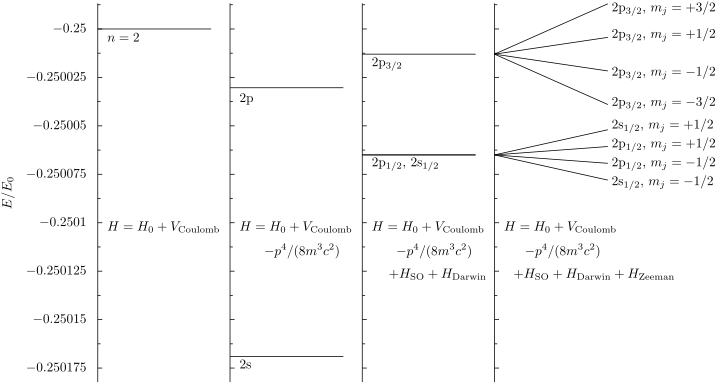
From left to right: energy levels of hydrogen with (a) Coulomb potential only, (b) Coulomb potential + relativistic correction, (c) Coulomb potential + all fine-structure corrections, and (d) Coulomb potential + fine structure + Zeeman effect terms.
The exact fine-structure energy levels of the hydrogen atom
The fine-structure corrections to the energy levels of hydrogen can also be calculated with the relativistic Dirac equation, which yield the fine-structure energy levels of the hydrogen atom without needing to invoke approximations. They are given by:
$$ E_{jn} = -m_{e}c^2 + m_{e}c^2\left( 1 + \left[ \frac{Z\alpha}{n - j - \frac{1}{2} + \sqrt{ \left( j + \frac{1}{2} \right)^2 - (Z\alpha)^2 }} \right]^2 \right)^{-1/2} $$
(Technically we should use the reduced mass $\mu$ instead of the electron mass $m_e$, though the substitution is straightforward.) Something very interesting happens if we Taylor-expand the exact solution from the Dirac equation, and this is sufficiently important that we will do it step-by-step. First, we use the Taylor series $(1 + x^2)^{-1/2} = 1 - \frac{1}{2}x^2 + \frac{3}{8}x^4 \dots$ to expand out the second term, giving us:
$$ \begin{align*} E_{jn} &\approx -m_{e}c^2 + m_{e}c^2\left\{ 1 - \frac{1}{2}\left[ \frac{Z\alpha}{n - j - \frac{1}{2} + \sqrt{ \left( j + \frac{1}{2} \right)^2 - (Z\alpha)^2 }} \right]^2 + \dots\right\} \\ &= \cancel{ -m_{e}c^2 } + \cancel{ m_{e}c^2 } -\frac{m_{e}c^2}{2} \left[ \frac{Z\alpha}{n - j - \frac{1}{2} + \sqrt{ \left( j + \frac{1}{2} \right)^2 - (Z\alpha)^2 }} \right]^2 + \dots \\ &= -\frac{m_{e}c^2(Z\alpha)^2}{2} \left[ \frac{1}{n - j - \frac{1}{2}+ \sqrt{ \left( j + \frac{1}{2} \right)^2 - (Z \alpha)^2 }} \right]^2 \\ &= -\frac{m_{e}c^2 (Z\alpha)^2}{2}\left[ n - \left( j + \frac{1}{2} \right) + \left( j + \frac{1}{2} \right)\sqrt{ 1 - \left(\small \frac{Z\alpha}{j + \frac{1}{2}} \right)^2 } \right]^{-2} \\ &\approx -\frac{m_{e}c^2 (Z\alpha)^2}{2}\left[ n - \left( j + \frac{1}{2} \right) + \left( j + \frac{1}{2} \right)\left( 1 - \frac{1}{2}\left(\small \frac{Z\alpha}{j + \frac{1}{2}} \right)^2 + \dots \right) \right]^{-2} \\ &= -\frac{m_{e}c^2 (Z\alpha)^2}{2} \left[ n - \cancel{ \left( j + \frac{1}{2} \right) } + \cancel{ \left( j + \frac{1}{2} \right) } -\frac{1}{2} \left( j + \frac{1}{2} \right)\left(\small \frac{Z\alpha}{j + \frac{1}{2}} \right)^2 + \dots \right]^{-2} \\ &= -\frac{m_{e}c^2 (Z\alpha)^2}{2n^2}\left[ 1 -\frac{1}{2n} \frac{(Z \alpha)^2}{\left( j + \frac{1}{2} \right)} + \dots \right]^{-2} \end{align*} $$
Here, in the first step, we perform our initial Taylor expansion; this naturally allows the $m_ec^2$ dependence to cancel out in the second step. Then, in the third step we factor out $(Z \alpha)^2$ from inside the fraction. In the fifth step, we factor out $\left(j + \frac{1}{2}\right)$ from the square root, which then allows us to use the following Taylor approximation:
$$ \sqrt{ 1 - \left(\small \frac{Z\alpha}{j + \frac{1}{2}} \right)^2 } = 1 - \frac{1}{2}\left(\small \frac{Z\alpha}{j + \frac{1}{2}} \right)^2 + \mathcal{O}((Z\alpha)^4) $$
Where $\mathcal{O}(Z^4\alpha^4)$ denotes terms that are fourth-order or higher in $Z\alpha$. This cancels out the first $j + \frac{1}{2}$ term, making the expression far simpler. Finally, in the last step, we factor out $n$ from the fraction. To finish, we use the binomial approximation $(1 - x)^{-2} \approx 1 + 2x$, giving us:
$$ \left[ 1 -\frac{1}{2n} \frac{(Z \alpha)^2}{\left( j + \frac{1}{2} \right)} + \dots \right]^{-2} \approx 1 + \frac{1}{n} \frac{(Z \alpha)^2}{\left( j + \frac{1}{2} \right)} $$
Plugging this in, our resulting energies become:
$$ E_{jn} \approx -\frac{m_{e}c^2 (Z\alpha)^2}{2n^2} \left[1 + \frac{1}{n} \frac{(Z \alpha)^2}{\left( j + \frac{1}{2} \right)} + \dots\right] $$
Which matches what we got from perturbation theory! Hence, the Dirac equation's solution reproduces the result from perturbation theory at low orders of $\alpha$. This is why the fine-structure constant is so important in quantum physics: it is the natural expansion parameter for perturbative expansions. Since $\alpha \ll 1$, higher powers of $\alpha$ become increasingly smaller, meaning that higher-power terms in series expansions involving $\alpha$ are much weaker. Hence, we can safely ignore higher-power terms when doing perturbative calculations. In contrast, if $\alpha \gg 1$, then higher-power terms in series expansions would actually grow increasingly larger, making perturbation theory useless. This phenomenon remains true even when we go into the world of quantum field theory, where the fine-structure constant occupies a fundamental role as the coupling constant of quantum electrodynamics!
Note: While the Dirac equation provides an exact solution for the energy levels due to fine-structure, it does not predict smaller effects, including hyperfine structure and the Lamb shift, which (respectively) arise due to nuclear structure and quantum electrodynamics. We will examine these effects shortly.
The hyperfine structure of hydrogen
Up to this point, we have considered the nucleus as a stationary point-like charge generating an electrostatic (Coulomb) potential, essentially like a classical point charge. However, we know now that this is not the case. Atomic nuclei are composed of protons and neutrons, which are also quantum particles. Crucially, atomic nuclei also have spin, and while nuclear spin can be neglected in a lot of problems, it is essential for explaining the hyperfine transitions of hydrogen.
The hyperfine transition occurs due to an interaction between the nuclear magnetic dipole moment and the magnetic field (in the nuclear rest frame) generated by the atomic electrons. Therefore, it is similar to spin-orbit coupling, except the spin is now nuclear spin, instead of electron spin. The nuclear magnetic dipole moment operator is given by:
$$ \boldsymbol{\mu}_{N} = g_I\frac{e}{2m_p} \hat{\mathbf{I}} = g_I \frac{\mu_{N}}{\hbar} \hat{\mathbf{I}} $$
Where $g_I$ is the nuclear spin g-factor, $m_{p}$ is the proton mass, $\mu_N$ is the nuclear magneton (a natural constant), and $\hat{\mathbf{I}}$ is the nuclear spin operator (similar to $\hat{\mathbf{S}}$, the electron spin operator). Since nuclei generally have both protons and neutrons, which have different masses, and may have different numbers of protons from neutrons, the nuclear g-factor does not have a simple formula (it is a constant that you generally have to look up). In the case of hydrogen, which has a nucleus made only of a single proton, $g_N \approx 5.6$.
In any case, the nuclear spin couples to the magnetic field generated by the electron. However, since the electron both has spin and orbital angular momentum, it has a more complicated magnetic field than a classical moving point charge. The orbital part of its magnetic field is straightforward: it is actually the same as what we used in calculating the spin-orbital contribution to fine structure, except we make the replacement $Ze \to -e$ to account for the different charge of the nucleus. This gives us the orbital magnetic field $\mathbf{B}_{\ell}$:
$$ \mathbf{B}_{\ell} = -\frac{e}{4\pi m_{e} \varepsilon_{0}c^2} \frac{\mathbf{L}}{r^3} = -\mu_{B} \frac{\mu_{0}}{2\pi} \frac{\mathbf{L}}{r^3} $$
Where $\mu_B = e\hbar/(2m_e)$ is the Bohr magneton. So far, so good; unfortunately, getting the contribution from the electron's spin is a much more complicated issue. This is because there is no classical analogue for spin. The closest approximation we can use is to model an electron as a magnetic dipole. The magnetic vector potential of a classical magnetic dipole is given by:
$$ \mathbf{A}(\mathbf{r}) = \frac{\mu_{0}}{4\pi} \frac{\mathbf{m} \times \mathbf{r}}{r^3} $$
Where $\mathbf{m}$ is the magnetic moment. The magnetic moment of an electron can be expressed as:
$$ \mathbf{m}_\mathrm{electron} = -\frac{g_{s}\mu_{B}\mathbf{S}}{\hbar} $$
Where $g_s \approx 2$ is the electron spin g-factor, $\mu_B$ is the Bohr magneton, and $\mathbf{S}$ is the spin angular momentum. The magnetic field is related to the magnetic vector potential by $\mathbf{B} = \nabla \times \mathbf{A}$, so the spin magnetic field $\mathbf{B}_{s}$ is:
$$ \mathbf{B}_{s} = \nabla \times \left( \frac{\mu_{0}}{4\pi} \frac{\mathbf{m} \times \mathbf{r}}{r^3} \right) = -\frac{g_{s} \mu_{0} \mu_{B}}{4\pi \hbar} \nabla \times \left( \frac{\mathbf{S} \times \mathbf{r}}{r^3} \right) $$
If we evaluate the curl here, it will expand to three terms:
$$ \nabla \times \left( \frac{\mathbf{S} \times \mathbf{r}}{r^3} \right) = \frac{3\mathbf{r}(\mathbf{S} \cdot \mathbf{r})}{r^5} - \frac{\mathbf{S}}{r^3} + \frac{8\pi}{3r^3} \delta^3(\mathbf{r}) \mathbf{S} $$
Where $\delta^3(\mathbf{r})$ is the 3-dimensional delta function. The total magnetic field from the electron is thus given by:
$$ \mathbf{B} = \mathbf{B}_{\ell} + \mathbf{B}_{s} $$
Now, we will construct the perturbation of the Hamiltonian describing hyperfine structure. As usual, when we go from a classical to quantum treatment, we replace the classical angular momentum $\mathbf{L}$ with its quantum counterpart, the angular momentum operator $\hat{\mathbf{L}}$. This gives us:
$$ \begin{align*} \Delta \hat{H}_\mathrm{hyperfine} &= -\boldsymbol{\mu}_{N} \cdot \mathbf{B} \\ &= -\boldsymbol{\mu}_{N} \cdot (\mathbf{B}_{\ell} + \mathbf{B}_{s}) \\ &= g_I \frac{\mu_{N}}{\hbar} \left\{ \mu_{B} \frac{\mu_{0}}{2\pi} \frac{\hat{\mathbf{L}} \cdot \hat{\mathbf{I}}}{r^3} + \frac{g_{s} \mu_{0} \mu_{B}}{4\pi \hbar} \hat{\mathbf{I}} \cdot \left[ \frac{3\mathbf{r}(\hat{\mathbf{S}} \cdot \mathbf{r})}{r^5} - \frac{\hat{\mathbf{S}}}{r^3} + \frac{8\pi}{3r^3} \delta^3(\mathbf{r}) \hat{\mathbf{S}} \right] \right\} \\ &= g_I \frac{\mu_{N}}{\hbar} \left\{ \mu_{B} \frac{\mu_{0}}{2\pi} \frac{\hat{\mathbf{L}} \cdot \hat{\mathbf{I}}}{r^3} + \frac{g_{s} \mu_{0} \mu_{B}}{4\pi \hbar r^3} \left[ \frac{3(\hat{\mathbf{I}} \cdot\mathbf{r})(\hat{\mathbf{S}} \cdot \mathbf{r})}{r^2} - \hat{\mathbf{I}} \cdot\hat{\mathbf{S}}+ \frac{8\pi}{3} \delta^3(\mathbf{r}) \hat{\mathbf{I}} \cdot\hat{\mathbf{S}} \right] \right\} \end{align*} $$
The delta function term is zero for $\ell = 0$, and evaluates to a term proportional to $|\psi(0)|^2$ otherwise. If one only computes the shifts for $\ell \neq 0$, we can can combine the term dependent on $\hat{\mathbf{L}} \cdot \hat{\mathbf{I}}$ and the term dependent on $\hat{\mathbf{I}} \cdot \hat{\mathbf{S}}$ into a single term dependent only on $\hat{\mathbf{J}}$, and apply the following identity:
$$ \hat{\mathbf{J}} \cdot \hat{\mathbf{I}} = \frac{\hbar^2}{2} [F(F + 1) - I(I + 1) - J(J + 1)] $$
Where $F = I + J$ is the total atomic angular momentum (as usual, $J = \ell + s$, we have simply written it with uppercase $J$ rather than lowercase $j$ as this is standard convention). We will not aim to calculate the general expressions for the energy corrections; that is left as an exercise for the reader, although the techniques are much the same as those we used to calculate the fine-structure corrections. Instead, we will simply give the result for the ground-state hyperfine corrections in hydrogen: it is:
$$ \Delta E = \frac{2}{3n^3}Z^4 \alpha^4 \left( \frac{m_{e}}{m_{p}} \right) (m_{e}c^2)g_I\left[ F(F + 1) - \frac{3}{2} \right] \quad (n = 1) $$
Since we are in the ground state ($n = 1, \ell = 0$) and the hydrogen nucleus (which is a single proton) always has a spin of $I = \frac{1}{2}$, the two possible states are $F = 0$ (spin-down) and $F = 1$ (spin-up). The ground-state hyperfine transition ($F = 1 \to F = 0$) is thus a spin-flip transition, where the electron goes from spin-up to spin-down, emitting a photon with an energy of $\Delta E \approx \pu{5.78 \mu eV}$. The hyperfine structure is an example of a so-called forbidden transition (the name is a misnomer because a "forbidden transition" really just means a transition is much less probable than a "allowed transition"). This originates from the (electric dipole coupling) selection rules for hydrogen, which mandate that for any transition, one has:
$$ \Delta \ell = \pm 1, \quad \Delta m = 0,\quad \Delta s = 0 $$
(This comes from the electric dipole transition that we'll calculate later on in time-dependent perturbation theory.) Normally, this means that a spin-flip transition is impossible, since we have a change of the spin quantum number. But in the hyperfine transition this is possible. However, it is far more unlikely; in fact a hyperfine transition happens (on average) once every 11 million years!
We can convert the hyperfine transition energy to frequency to find that a photon emitted (or absorbed) as a result of a hyperfine transition has a frequency of $\pu{1.42 GHz}$ (or more precisely, $1.420405751768(2) \text{{ GHz}}$, a value that has been measured to incredible precision). Converted to wavelength, this results in a wavelength of $\lambda \approx \pu{21 cm}$, which is in the microwave range of the electromagnetic spectrum.
While hyperfine splitting may seem like a tiny quantum correction that barely matters, it actually has tremendous importance in timekeeping and astronomy. The 21-centimeter spectral line of hydrogen is found almost everywhere in outer space, due to the prevalence of hydrogen in the Universe (particularly in hydrogen gas clouds), and observations of the 21 cm line were responsible for revealing the spiral structure of our galaxy. Hydrogen masers (microwave lasers) used for precision interferometry and in atomic clocks rely on the hyperfine transition and are used as some of the most accurate clocks because of the highly-stable frequency of the beams they emit.
Order of magnitude of fine and hyperfine energy corrections
It is instructive to ask the question: how do fine structure and hyperfine structure compare in the relative magnitudes? First of all, both effects are to the same order in $\alpha$, the fine structure constant. Specifically, they are of order $\mathcal{O}(\alpha^4)$ in magnitude, which tells us that they are at least weaker by a factor of $\alpha^2$ than the electronic transitions (unperturbed energy levels) of the hydrogen atom, which are $\mathcal{O}(\alpha^2)$. This explains why we can afford to neglect fine (and hyperfine) structure in the hydrogen atom while still predicting spectral lines to good accuracy. However, this is not the full story: the energies associated with hyperfine transitions are much smaller in magnitude than that of fine structure transitions, since they also depend on the ratio $m_e/m_p \approx \frac{1}{1836}$ of the electron mass to the proton mass. Hence, hyperfine transitions are typically suppressed by lower-order effects and are not easily observed. The table below gives an overview of the comparison between electronic, fine-structure, and hyperfine transitions:
| Transition | Typical energy splitting | Type of EM radiation emitted |
|---|---|---|
| Electronic (unperturbed) | Around $\pu{1 eV - 10 eV}$ | UV, visible light, near-infrared |
| Fine structure | Around $\pu{1 meV}$ | UV, visible light, near-infrared |
| Hyperfine structure | Around $\pu{1 \mu eV}$ | Microwaves (GHz range) |
The Lamb shift
Although fine (and hyperfine) structure lifts the degeneracy of many of the states of the hydrogen atom, it does not do so for all of them. For instance, the transition $2s^{1/2} \to 2p^{1/2}$ is conventionally impossible since they share the same $n$ and $j$ quantum numbers; hence, the fine-structure formula would tell us that the two states are degenerate (and thus share the same energies). Nevertheless, we physically do observe the transition, and it is due to something called the Lamb shift.
The Lamb shift originates from the quantum fluctuations of the electromagnetic field, much like the Darwin term in our calculation of the fine structure. Roughly-speaking, the quantum fluctuations have the net effect of "smearing" out the electron's position, which in turn modifies the Coulomb potential:
$$ V(r) = -\frac{Qe^2}{4\pi \varepsilon_{0}r} \to -\frac{Qe^2}{4\pi \varepsilon_{0}(r + \delta r)} $$
Where $\delta r$ is the average size of the fluctuations and $Q = Z$. While a full derivation of the Lamb shift would require relativistic quantum field theory (which is something we'll cover much later), we can use a non-relativistic approximation to calculate the Lamb shift in the context of perturbation theory. The precise details are a bit complex (see these lecture notes if you want to see the derivation), but the general result is:
$$ \Delta E_{n} = \frac{2\alpha}{3\pi m_{e}^2 c^2} \frac{\hbar^2 \ln(k_0)}{2} \langle \nabla^2 V_{C}\rangle $$
Where $V_{C} = -Ze^2/4\pi \varepsilon_0 r$ is the Coulomb potential and $\ln(k_0) \approx \ln(1/8.9 \alpha^2)$ is known as the Bethe logarithm. To compute the energy shifts explicitly, we must compute $\langle \nabla^2 V_{C}\rangle$. The following identity is useful:
$$ \nabla^2\left( \frac{1}{r} \right) = -4\pi \delta^3(\mathbf{r}) $$
Where $\delta^3(r)$ is the 3-dimensional Dirac delta function. Thus we have:
$$ \langle \nabla^2 V\rangle = -\frac{Z e^2}{4\pi\varepsilon_{0}} \int \psi_{n}^*(\mathbf{r}) \delta(\mathbf{r}) \psi_{n}(\mathbf{r}) dV = -\frac{Z e^2}{\varepsilon_{0}}|\psi_{n}(0)|^2 $$
In the case of hydrogen and similar atoms, we know that the wavefunction at the origin is only nonzero for $\ell = m = 0$, for which it is given by:
$$ |\psi_{n00}(0)|^2 = \frac{1}{\pi} \left( \frac{Z}{na_{0}} \right)^3 = \frac{1}{\pi} \left( \frac{Z}{n} \frac{\alpha m_{e}c}{\hbar} \right)^3 $$
Substituting this back into our expression for $\Delta E_n$, we have:
$$ \begin{align*} \frac{\hbar^2}{2} \langle \nabla^2 V\rangle &= -\frac{Ze^2 \hbar^2}{2 \varepsilon_{0}} |\psi_{n}(0)|^2 \\ &= -\frac{Z^4e^2 \hbar^2}{2\pi \varepsilon_{0} n^3} \left(\frac{\alpha m_{e}c}{\hbar} \right)^3 \\ &= Z^4 \hbar^2 \left( \frac{2\hbar c \alpha}{n^3} \right) \left( \frac{\alpha m_{e}c}{\hbar} \right)^3 \\ &= \frac{2Z^4 \alpha^4}{n^3} m_{e}^3 c^4 \end{align*} $$
Where it is useful to note that $\frac{e^2}{2\pi \varepsilon_{0}} = 2\hbar c \alpha$. Hence, the energy shifts are given by:
$$ \Delta E_{n} = \frac{2\alpha}{3\pi m_{e}^2 c^2} \frac{2Z^4 \alpha^4}{n^3} m_{e}c^4\ln(k_0) = \frac{4Z^4\alpha^5 m_{e}c^2}{3\pi n^3} \ln k_{0} \approx \pu{34.37 \mu eV} \cdot\frac{Z^4}{n^3} $$
For the transition $2s^{1/2} \to 2p^{1/2}$, this corresponds to a frequency of $\nu \approx \pu{1085.15 MHz}$, which is within 3% of the experimentally measured value of $\pu{1057.864 MHz}$. This is a tiny energy difference many orders of magnitude below that of electronic energy levels, which explains why we typically don't notice the Lamb shift. Indeed, since it depends on $\alpha^5$ it is an order of magnitude smaller than fine structure, which depends on $\alpha^4$. However, notice that the Lamb shift also grows with the fourth power of the atomic number. Hence, while the Lamb shift is an extremely tiny correction to the energy levels of the hydrogen atom and is usually negligible, it can become a much larger energy shift for super-heavy atoms (e.g. uranium), for which it cannot be ignored.
We will now account for the discrepancy between our theoretically-predicted transition frequency and the experimental data. This discrepancy comes as a result of several factors: first, our treatment is non-relativistic, and second, it includes only the so-called self-energy correction. There are two other smaller effects that contribute towards the Lamb shift, as shown below:
| Effect | Energy contribution |
|---|---|
| Electron self-energy* | +1017 MHz |
| Anomalous magnetic moment | +68 MHz |
| Vacuum polarization | -27 MHz |
| Total | +1058 MHz |
Source: LibreTexts
*: Also known as "electron mass renormalization" in the quantum electrodynamics
The effect of vacuum polarization can be described by replacing the Coulomb potential with a modified potential in the form:
$$ \begin{align*} V(r) &= -\frac{Ze^2}{4\pi\varepsilon_{0}}\left( 1 + \frac{4}{15} \left( \frac{e^2 \hbar^3}{4\pi \varepsilon_{0} m_{e}^2 c} \right) \delta^{(3)}(r) \right) \\ &= -\left( \frac{\alpha \hbar c}{r} + \frac{4\alpha^2 \hbar^3}{15m_{e}^2 c} \delta^{(3)}(r) \right) \end{align*} $$
Where $\alpha$ is the fine-structure constant and $\delta^{(3)}(r)$ is the 3-dimensional Dirac delta function (for those curious, see Quantum Field Theory for the Gifted Amateur Ch. 41.1 for the derivation from the renormalized photon propagator). The second term in the potential can be treated as a perturbation $\Delta V$ to the potential, that is:
$$ \Delta V = -\frac{4\alpha^2 \hbar^3}{15m_{e}^2 c} \delta^{(3)}(r) $$
Using first-order perturbation theory with this as our perturbation gives us an energy shift of:
$$ \Delta E = \int \psi_{n}^*(\mathbf{r}) \Delta V \psi_{n}(\mathbf{r})dV = -\frac{4\alpha^2 \hbar^3}{15m_{e}^2 c} |\psi(0)|^2 =-\frac{4\alpha^2 \hbar^3}{15\pi m_{e}^2 c} \left( \frac{Z}{na_{0}} \right)^3 $$
Finally, the effect of the anomalous magnetic moment can be incorporated by replacing $g_{s} = 2$ in the spin-orbital coupling terms in the Hamiltonian with the actual value of $g_s = 2 + \frac{\alpha}{\pi} + \dots$ which is approximately $g_{s} = 2.0023193$. For those curious, this effect comes from the non-trivial terms in the QED vertex function, but that is beyond the scope of this guide. Finally, while our computation predicts that the Lamb shift is only nonzero for $s$ orbitals, we do observe a (much smaller) shift for $p$ orbitals as well; this suggests that we have to be more careful with our approximations. A detailed calculation of the Lamb shift using relativistic quantum field theory leads to a result that differs from the experimental value by under $10^{-6}$, making it one of the most accurate predictions in all of physics.
The variational method
Perturbation theory is all well and good for finding approximate solutions to the Schrödinger equation, but it is not perfect. This is because it requires an arbitrary Hamiltonian to be able to be written as the sum of a simple, analytically-solvable Hamiltonian plus a small perturbation. It no longer works if the perturbation is large, or if this decomposition is not possible!
However, this does not mean we are out of options! Indeed, physicists have developed a variety of other techniques to solve problems that neither perturbation theory nor exact analytical methods can handle. One of these methods is called the variational method. This comes from the fact that one can show that the true ground-state energy $E_0$ associated with any Hamiltonian $\hat H$ satisfies the following inequality:
$$ E_{0} \leq \frac{\langle \psi_{0} |\hat{H} | \psi_{0}\rangle}{\langle \psi |\psi\rangle} $$
If $|\psi_0\rangle$ normalized, that is, $|\langle \psi_0|\hat H|\psi_0\rangle|^2$, this reduces to the simplified form:
$$ E_{0} \leq \langle \psi_{0} |\hat{H} | \psi_{0}\rangle $$
If we are working in the position basis, this can be rewritten as:
$$ E_{0} \leq \frac{\displaystyle \int \psi_{0}^*(\mathbf{r}) \hat{H} \psi_{0}(\mathbf{r}) d\tau}{\displaystyle \int \psi_{0}^*(\mathbf{r}) \psi_{0}(\mathbf{r}) d\tau} $$
Where $d\tau$ is the integration element (e.g. $dx$ in 1D Cartesian coordinates, $dxdy$ in 2D Cartesian coordinates, $dx dy dz$ in 3D, $r^2 d r d\Omega$ in spherical coordinates, etc.). This reduces to the following if $\psi_0$ is normalized:
$$ E_{0} \leq \int \psi_{0}^*(\mathbf{r}) \hat{H} \psi_{0}(\mathbf{r}) d\tau $$
This immediately makes the problem of finding the ground-state wavefunctions (and energies) a minimization problem (or, in the language of mathematicians, a variational problem). What we can then do is to guess a wavefunction parameterized in terms of one or more constant parameters $\gamma$:
$$ \psi_{0}(\mathbf{r}) = \psi_{0}(\mathbf{r}; \gamma), \quad \gamma = (a, b, c, \dots, \gamma_{n}) $$
Where the integral is over the entire domain over which the ground-state wavefunction is defined. To find the values of the parameters $a, b, c, \dots$ we can use a classic method from multivariable calculus. Recall that for a function of several variables, its minima are located at its critical points, where the first derivatives of the function are all zero. Hence, to minimize the energy of the ground state, we set the first derivatives of the ground-state wavefunctions with respect to the parameters equal to zero:
$$ \frac{\partial}{\partial (\text{params})} \left(\frac{\langle \psi_{0} |\hat{H} | \psi_{0}\rangle}{\langle \psi |\psi\rangle}\right) = 0 $$
Expanding this, we can rewrite the above as:
$$ \begin{align*} \frac{\partial \psi_{0}}{\partial a} &= 0 \\ \frac{\partial \psi_{0}}{\partial b} &= 0 \\ \frac{\partial \psi_{0}}{\partial c} &= 0 \\ \vdots &\quad \vdots \\ \frac{\partial \psi_{0}}{\partial \gamma_{n}} &= 0 \end{align*} $$
From here, we get a system of equations, which can be solved to find the values of $a, b, c, \dots$ that would minimize $\dfrac{\langle\psi_{0} |\hat{H} | \psi_{0}\rangle}{\langle \psi_{0}|\psi_{0}\rangle}$ (which is called the energy functional and which we will denote as $\varepsilon$). Once this is done, we can substitute those parameters back into $\psi_0$, which will (hopefully) have a good approximation of the ground-state energy:
$$ E_{0} \approx \varepsilon = \frac{\langle\psi_{0} |\hat{H} | \psi_{0}\rangle}{\langle \psi_{0}|\psi_{0}\rangle} $$
This technique is powerful because it does not rely on $\hat H$ being able to be separated into a small perturbation on top of a simpler Hamiltonian. However, the accuracy of the approximate ground-state energy obtained from the variational method may greatly vary, depending on how many parameters we put (more parameters generally makes the approximation more accurate) and how close our guess for $\psi_0$ is to the true ground-state wavefunction.
Note: Typically-speaking, the variational method can only compute the ground-state wavefunction and ground-state energy of a system. However, it is possible to find (or at least) estimate the higher-energy states (excited states) of a system using the Gram–Schmidt algorithm.
Solving the hydrogen atom by the variational method
Let us return to the hydrogen atom, whose Hamiltonian, as we saw, is given by:
$$ H = -\frac{\hbar^2}{2\mu} \nabla^2 - \frac{Ze^2}{4\pi \varepsilon_{0} r} $$
With $\mu$ being the reduced mass and $Z$ being the atomic number, and where we use $q$ for the electron's charge. We will use the variational method to attempt to approximate the ground-state energy and ground-state wavefunction of the hydrogen atom. We will rewrite this as:
$$ H = b_{1} \nabla^2 + \frac{b_{2}}{r}, \quad b_{1} = -\frac{\hbar^2}{2\mu}, \quad b_{2} = -\frac{Ze^2}{4\pi \varepsilon_{0}} $$
Next, we choose the following ansatz (educated guess) for the ground-state wavefunction:
$$ \psi_{0}(r) = a e^{-r /\lambda} $$
Where $a$ and $\lambda$ are unknown constants. We can justify this heuristically: we know that the wavefunction must be normalizable and that it must be well-defined for all real numbers: this suggests a function that smoothly decays to zero at infinity. Moreover, we know that it must be spherically-symmetric due to the spherical symmetry of the hydrogen atom. The above ansatz satisfies all the above: the $e^{-r/\lambda}$ decay ensures a smooth decay as $r \to \infty$ and is normalizable, and moreover it is only dependent on $r$, making it spherically-symmetric. In addition — and this is especially important when doing calculations by hand — it is reasonably simple, hence calculating the resulting integrals will be less of a nightmare. We can always add more parameters later. It is useful to note the following identities:
$$ \begin{gather*} \frac{d}{dr} e^{-r / \lambda} = -\frac{1}{\lambda} e^{-r/\lambda}, \quad \frac{d^2}{dr^2} e^{-r / \lambda} = \frac{1}{\lambda^2} e^{-r / \lambda} \\ \nabla^2 f(r) = \frac{1}{r^2} \frac{d}{dr}\left( r^2 \frac{d f}{dr} \right) = \frac{2}{r} \frac{df}{dr} + \frac{d^2 f}{dr^2} \end{gather*} $$
Where $f(r)$ is any spherically-symmetric function of purely the radial coordinate $r$. Substituting into the Hamiltonian, and computing the derivatives, we have:
$$ \begin{align*} \hat H \psi_{0} &= \left[b_{1} \nabla^2 + \frac{b_{2}}{r}\right] \psi_{0}(r) \\ &= b_{1}\left( \psi_{0}'' + \frac{2}{r} \psi_{0}' \right) + \frac{b_{2}}{r} \psi_{0} \\ &= \frac{ab_{1}}{\lambda^2} e^{-r / \lambda} - \frac{2ab_{1}}{\lambda} \frac{e^{-r / \lambda}}{r} + \frac{ab_{2}}{r} e^{-r / \lambda} \\ &= a \left\{\frac{b_{1}}{\lambda^2} + \frac{1}{r} \left[ b_{2} - \frac{2b_{1}}{\lambda} \right] \right\}e^{-r / \lambda} \end{align*} $$
Hence, we obtain (upon integrating in spherical coordinates):
$$ \begin{align*} \langle \psi_{0} | \hat{H} | \psi_{0} \rangle &= \int_{0}^{2\pi} \int_{0}^\pi \int_{0}^\infty \psi_{0}(r) \hat{H} \psi_{0}(r) r^2 \sin \theta dr d\theta d \phi \\ &= 4\pi \int_{0}^\infty \psi_{0}(r) \hat{H} \psi_{0}(r) r^2 dr \\ &= 4\pi a^2 \int_{0}^\infty \left\{\frac{b_{1}}{\lambda^2} + \frac{1}{r} \left[ b_{2} - \frac{2b_{1}}{\lambda} \right] \right\}e^{-2r / \lambda} r^2 dr \\ &= \pi a^2 \left( \frac{b_{1}}{\lambda^2} \lambda^3 + \left[ b_{2} - \frac{2b_{1}}{\lambda} \right]\lambda^2 \right) \\ &=\pi a^2 (b_{1}\lambda + b_{2}\lambda^2 -2b_{1}\lambda) \\ &= \pi a^2 (b_{2}\lambda^2 - b_{1}\lambda) \\ \langle \psi_{0} | \psi_{0}\rangle &= \int_{0}^{2\pi} \int_{0}^\pi \int_{0}^\infty |\psi_{0}|^2 r^2 \sin \theta dr d\theta d\phi \\ &= 4\pi \int_{0}^\infty a^2 e^{-2r /\lambda}r^2 dr \\ &= \pi a^2 \lambda^3 \\ &= 1 \end{align*} $$
Where we used the following identities (both can be derived from integration by parts):
$$ \int_{0}^\infty re^{-2r/\lambda} dr = \frac{\lambda^2}{4}, \quad \int_{0}^\infty r^2 e^{-2r / \lambda} dr = \frac{\lambda^3}{4} $$
Thus, the energy functional $\varepsilon$ is given by:
$$ \varepsilon = \frac{\langle\psi_{0} |\hat{H} | \psi_{0}\rangle}{\langle \psi_{0}|\psi_{0}\rangle} = \frac{\pi a^2 (b_{2}\lambda^2 - b_{1}\lambda)}{\pi a^2 \lambda^3} = \frac{b_{2}}{\lambda} - \frac{b_{1}}{\lambda^2} $$
In this case, we would conventionally differentiate with respect to both $a$ and $\lambda$ to get our system of equations. But we are fortunate that the normalization procedure has already told us that $\pi a^2 \lambda^3 = 1$, hence $a = 1 / \sqrt{\pi \lambda^3}$. Therefore, we only need to minimize with respect to $\lambda$. Taking the derivative with respect to $\lambda$ and setting it equal to zero yields:
$$ \frac{d\varepsilon}{d\lambda} = -\frac{b_{2}}{\lambda^2} + \frac{2b_{1}}{\lambda^3} = 0 $$
We can now solve for the value of $\lambda$ that satisfies the above equation, which is just a matter of some straightforward algebra. The solution is:
$$ \lambda = \frac{2 b_{1}}{b_{2}} = \frac{4\pi \varepsilon_{0} \hbar^2}{Z \mu e^2} = \frac{a_{0}^*}{Z} $$
Where $a_{0}^* = \frac{m_{e}}{\mu} a_{0}$ is the reduced Bohr radius, and $a_0 \approx \pu{5.29 * 10^{-11} m}$ is the Bohr radius, as we saw in the derivation of the hydrogen atom. Thus we find that $\lambda = a_0^* / Z$, the Bohr radius, while $a = 1/\sqrt{\pi \lambda^3}$. Substituting back into our ansatz $\psi_{0}(r) = a e^{-r /\lambda}$ gives us a ground-state wavefunction of:
$$ \psi_{0} = \frac{1}{\sqrt{ \pi }} \left( \frac{Z}{a_{0}^*} \right)^{3/2} e^{-Zr / a_{0}^*} $$
This is actually the exact ground-state wavefunction of hydrogen! Thus, using the variational method, we were able to derive the ground-state wavefunction without needing to solve complicated differential equations. In addition, if we substitute our parameters into the energy functional, we get an estimated ground-state energy of:
$$ \begin{align*} \varepsilon &= \frac{b_{2}}{\lambda} - \frac{b_{1}}{\lambda^2} \\ &= -Z^2\left( \frac{e^2}{4\pi \varepsilon_{0} a_{0}^*} + \frac{\hbar^2}{2\mu {a_{0}^*}^2} \right), \quad a_{0}^*= \frac{4\pi \varepsilon_{0} \hbar^2}{\mu e^2} \\ &= -\frac{Z^2 \mu e^4}{32\pi^2 \varepsilon_{0}^2 \hbar^2} \\ & \approx -(\pu{13.6 eV})Z^2 \end{align*} $$
We know this is indeed the correct ground-state energy of hydrogen! In this particular case, we got lucky, since our ansatz happened to exactly match the hydrogen ground-state wavefunction and hence the variational method gave us an exact answer. Usually, we'll end up with an approximate answer instead of an exact one, albeit an answer that is "good enough" to approximate the ground-state energy pretty well.
Solving the helium atom by the variational method
As we mentioned earlier in the guide, the solution for the hydrogen atom is only valid for atoms with a single electron. While it can approximately describe multi-electron atoms, its predicted energy levels are not very accurate. This is because our treatment does not include a variety of effects in multi-electron atoms that affect the total energy:
- Nuclear screening, which comes from the inner electrons forming a negatively-charged "cloud" around the nucleus
- Electron correlation, which comes from inter-electron interactions within the atom, due to their electrostatic repulsion
- The exchange interaction, which comes from the Pauli exclusion principle that forbids electrons from sharing the same quantum state, causing electron-electron repulsion
The next-simplest atom after hydrogen is the helium atom, composed of 2 protons, (usually) 2 neutrons, and 2 electrons. The solution for the hydrogen atom can easily be generalized to helium by setting $Z = 2$. This would give us a predicted ground-state energy of:
$$ E_\mathrm{predicted} = -\pu{54.4228 eV} $$
Unfortunately, this is quite a bit off from the experimental value, and the reason is because the helium Hamiltonian has a different form from the hydrogen Hamiltonian. In particular, the helium Hamiltonian (disregarding spin and fine/hyperfine-structure corrections) is given by:
$$ \hat H = \underbrace{-\dfrac{\hbar^2}{2\mu}(\nabla_1^2 + \nabla_2^2)}_\text{electron kinetic energy} -\underbrace{\dfrac{Z}{4\pi \varepsilon_0}\left(\dfrac{e^2}{|\mathbf{r}_1|} + \dfrac{e^2}{|\mathbf{r}_2|}\right)}_\text{nucleus-electron attraction} + \underbrace{\dfrac{1}{4\pi \varepsilon_0}\dfrac{e^2}{|\mathbf{r}_1 - \mathbf{r}_2|}}_\text{electron-electron repulsion} $$
Where $Z = 2$ (since helium has two protons), $\mathbf{r}1 = (r{1}, \theta_{1}, \phi_{1})$ and $\mathbf{r}2 = (r{2}, \theta_{2}, \phi_{2})$ are the position coordinates for each of the two electrons and $\nabla_1^2, \nabla_2^2$ are respectively the Laplacians with respect to the coordinates $\mathbf{r}_1$ and $\mathbf{r}_2$. The first 4 terms in the helium Hamiltonian are more or less familiar: they are just the kinetic and potential terms for the first and second electron in helium. However, it is the last term that matters to us. This is the electron correlation term and it means that no analytical solution can be found for helium. Hence, we must tackle the problem using variational techniques.
To start, we choose the following ansatz for the ground-state wavefunction with two parameters, $Z_e$ and $\lambda$:
$$ \psi_{0}(\mathbf{r}_{1}, \mathbf{r}_{2}) = \frac{Z_{e}^3}{\pi \lambda^3} e^{-Z_{e}(r_{1} + r_{2}) / \lambda} $$
This is similar with our ansatz for the hydrogen atom ($\psi_{0}(r) = a e^{-r /\lambda}$, where we found that $a = \sqrt{\pi \lambda^3}$ and $\lambda = a_0^*/Z$). In fact, it is almost equal to the product of two hydrogen ground-state wavefunctions, with the exception of replacing $Z$ by $Z_e$, which represents an effective nuclear charge. We would expect that the negatively-charged electrons would counter the positive charge of the nucleus, resulting in a lower effective nuclear charge $Z_{e} < Z$ (in the case of helium specifically, this reduces to $Z_e < 2$).
Now, we can begin the variational procedure. First, we need to compute $\hat H \psi_{0}$. This becomes more complicated due to the electron correlation term, which is the magnitude of a difference of vectors; hence we must rewrite it in explicitly terms of coordinates. For this, we can use the well-known identity (which comes from the law of cosines):
$$ |\mathbf{r}_1 - \mathbf{r}_2| = \sqrt{ r_{1}^2 + r_{2}^2 + 2 r_{1}r_{2} \cos \theta_{2} } $$
It is also useful to use the following identity when computing the Laplacians $\nabla_1^2, \nabla_2^2$:
$$ \nabla_{i}^2 \psi(r) = \frac{2}{r} \frac{d\psi}{dr_{i}} + \frac{d^2 \psi}{dr_{i}^2} $$
Hence we have:
$$ \nabla_1^2 \psi(r) = \frac{2}{r} \frac{d\psi}{dr_{1}} + \frac{d^2 \psi}{dr_{1}^2}, \quad \nabla_{2}^2 \psi(r) = \frac{2}{r} \frac{d\psi}{dr_{2}} + \frac{d^2 \psi}{dr_{2}^2} $$
It is recommended to perform the remainder of the calculation with a computer algebra system such as Maple, Mathematica, or SymPy as the calculations get quite involved: we will state just the general steps. However, while tedious, the math is just a combination of differentiation, integration, and algebra. There will be no need to solve differential equations or eigenvalue equations. This is part of the beauty of the variational method: it allows you to find the ground-state wavefunction and energy by performing a series of explicit steps, removing the guesswork from the problem (as long as you have already come up with an ansatz). Just substitute everything into the helium Hamiltonian, which will give you (after some simplifications and moving terms around) the following:
$$ \begin{align*} \hat{H} \psi_{0} &= \underbrace{ \left[-\frac{\hbar^2}{2\mu}(\nabla_{1}^2 + \nabla_{2}^2 ) - \frac{e^2}{4\pi \varepsilon_{0}}\left( \frac{Z_{e}}{r_{1}} + \frac{Z_{e}}{r_{2}} \right)\right] \psi_{0} }_{\hat{H}_{1}} \\ &\qquad + \underbrace{ \frac{e^2}{4\pi\varepsilon_{0}}\left[ \frac{Z_{e} - Z}{r_{1}} + \frac{Z_{e} - Z}{r_{2}}\right] \psi_{0} }_{\hat{H}_{2}} + \underbrace{ \frac{e^2}{4\pi\varepsilon_{0}} \frac{1}{|\mathbf{r}_{1} - \mathbf{r}_{2}|} \psi_{0} }_{\hat{H}_{3}} \end{align*} $$
Notice how we have written the Hamiltonian as a sum of three distinct terms: this will be important shortly. Next, we'll compute $\langle \psi_0 |\hat H|\psi_0\rangle$. We could brute-force it by plugging everything into the formula, but there is a clever and faster way. Notice that the Hamiltonian is linear in $\psi_{0}$ and has three terms; hence its eigenvalue equation can also be written in the following three-term form:
$$ \langle \psi_{0}|\hat{H} |\psi_{0}\rangle = (\hat{H}_{1} + \hat{H}_{2} + \hat{H}_{3})|\psi_{0}\rangle = (A E_\mathrm{hydrogen} + E_\mathrm{screening} + E_\mathrm{correlation})|\psi_{0}\rangle $$
Where $E_\mathrm{hydrogen} = -\pu{13.6 eV}$ is the ground-state energy of hydrogen and $A$ is a to-be-determined constant; the reasoning for the energies will be explained shortly. If we take the inner product with $\langle \psi_{0}|$ we get:
$$ \begin{align*} \langle \psi_{0} | \hat{H}_{1} | \psi_{0}\rangle &= A E_\mathrm{hydrogen} \\ \langle \psi_{0} | \hat{H}_{2} | \psi_{0}\rangle &= E_\mathrm{screening} \\ \langle \psi_{0} | \hat{H}_{3} | \psi_{0}\rangle &= E_\mathrm{correlation} \\ \end{align*} $$
This gives us the three following equations, upon expanding the inner product:
$$ \begin{align*} \int \psi_{0}\left[-\frac{\hbar^2}{2\mu}(\nabla_{1}^2 + \nabla_{2}^2 ) - \frac{e^2}{4\pi \varepsilon_{0}}\left( \frac{Z_{e}}{r_{1}} + \frac{Z_{e}}{r_{2}} \right)\right] \psi_{0}\,dV_{1} dV_{2} &= A E_\mathrm{hydrogen} \\ \int \psi_{0}\frac{e^2}{4\pi\varepsilon_{0}}\left[ \frac{Z_{e} - Z}{r_{1}} + \frac{Z_{e} - Z}{r_{2}}\right] \psi_{0}\, dV_{1} dV_{2} &= E_\mathrm{screening} \\ \int \psi_{0}\frac{e^2}{4\pi \varepsilon_{0}} \frac{1}{|\mathbf{r}_{1} - \mathbf{r}_{2}|} \psi_{0}\, dV_{1} dV_{2} &= E_\mathrm{correlation} \end{align*} $$
(Where $dV_i = r_i^2 dr_i d\theta_i d\phi_i$ and we integrate over a 6-dimensional domain for all $r_1, r_2, \theta_1, \theta_2, \phi_1, \phi_2$) We observe that the first equation is effectively two "copies" of the hydrogen Hamiltonian (except with respect to different coordinates, and with $Z$ replaced by $Z_e$). Hence, the energy eigenvalue must be twice that predicted by the ground-state energy formula for hydrogen (which is given by $E_0 = -Z^2 \cdot \pu{13.6 eV}$; here we'll have to replace $Z$ with $Z_e$). That is to say:
$$ AE_\mathrm{hydrogen} = 2 \cdot(-Z_{e}^2 \cdot \pu{13.6 eV}) = 2Z_{e}^2 \cdot E_\mathrm{hydrogen} \implies A = -2Z_{e}^2 $$
Hence, we have:
$$ \langle \psi_{0} | \hat{H}_{1} | \psi_{0}\rangle = 2Z_{e}^2 E_\mathrm{hydrogen} $$
For the second term, we will now evaluate the integral:
$$ \begin{align*} E_\mathrm{screening} &= \frac{e^2}{4\pi\varepsilon_{0}}\int \psi_{0}\left[ \frac{Z_{e} - Z}{r_{1}} + \frac{Z_{e} - Z}{r_{2}}\right] \psi_{0}\, dV_{1} dV_{2} \\ &= \frac{e^2}{4\pi\varepsilon_{0}} \left( \frac{Z_{e}^3}{\pi \lambda^3} \right)^2 \int_{0}^{2\pi} \int_{0}^\pi \int_{0}^\infty\int_{0}^{2\pi} \int_{0}^\pi \int_{0}^\infty e^{-2Z_{e}(r_{1} + r_{2}) / \lambda} \\ &\qquad \times \left[ \frac{Z_{e} - Z}{r_{1}} + \frac{Z_{e} - Z}{r_{2}}\right] r_{1}^2 \sin \theta_{1} d\theta_{1} d\phi_{1} ~ r_{2}^2 \sin \theta_{2} d\theta_{2} d\phi_{2} \end{align*} $$
What looks like a horrible integral is made immediately-easier by spherical symmetry, meaning that:
$$ \int_{0}^{2\pi} \int_{0}^\pi \sin \theta_{1} d \theta_{1} d\phi_{1} = \int_{0}^{2\pi} \int_{0}^\pi \sin \theta_{2} d \theta_{2} d\phi_{2} = 4\pi $$
Hence, four of the six integrals reduce down to a factor of $(4\pi)^2$, giving us:
$$ \begin{align*} E_\mathrm{screening} &= \frac{e^2}{4\pi\varepsilon_{0}} \left( \frac{Z_{e}^3}{\pi \lambda^3} \right)^2(4\pi)^2 \int_{0}^\infty \left[ \frac{Z_{e} - Z}{r_{1}} + \frac{Z_{e} - Z}{r_{2}}\right]e^{-2Z_{e}(r_{1} + r_{2}) / \lambda}r_{1}^2 dr_{1} r_{2}^2 dr_{2} \\ &= \frac{e^2}{4\pi\varepsilon_{0}} \left( \frac{Z_{e}^3}{\pi \lambda^3} \right)^2(4\pi)^2 \int_{0}^\infty \left( r_{1}(Z_{e} - Z) r_{2}^2 + r_{2}(Z_{e} - Z) r_{1}^2 \right) e^{-2Z_{e}(r_{1} + r_{2}) / \lambda} dr_{1} dr_{2} \\ &= 2(Z_{e} - Z)\left( \frac{Z_{e}e^2}{4\pi \varepsilon_{0} \lambda} \right), \quad \lambda = a_{0}^* \end{align*} $$
Which can be written in terms of $E_\mathrm{hydrogen}$ as:
$$ E_\mathrm{screening} =-4Z_{e}(Z_{e} - Z) E_\mathrm{hydrogen} $$
The final (and most challenging) integral to perform is the third term, which, unlike the others, does have angular dependence. It is given by:
$$ \begin{align*} E_\mathrm{correlation} &= \int \psi_{0}\frac{e^2}{4\pi \varepsilon_{0}} \frac{1}{|\mathbf{r}_{1} - \mathbf{r}_{2}|} \psi_{0}\, dV_{1} dV_{2} \\ &= \frac{e^2}{4\pi \varepsilon_{0}} \left(\frac{Z_{e}^3}{\pi \lambda^3} \right)^2 \int \frac{e^{-Z_{e}(r_{1} + r_{2}) / \lambda}}{\sqrt{ r_{1}^2 + r_{2}^2 + 2 r_{1}r_{2} \cos \theta_{2} }} dV_{1} dV_{2} \\ &= \frac{5Z_{e}}{8a_{0}^*} \left( \frac{e^2}{4\pi \varepsilon_{0}} \right) \\ &= -\frac{5Z_{e}}{4} E_\mathrm{hydrogen} \end{align*} $$
Therefore, putting all the terms together, we obtain:
$$ \begin{align*} \langle \psi_{0}|\hat{H} |\psi_{0}\rangle &= A E_\mathrm{hydrogen} + E_\mathrm{screening} + E_\mathrm{correlation} \\ &= \left( 2Z_{e}^2 - 4Z_{e}(Z_{e} - Z) - \frac{5}{4}Z_{e} \right) E_\mathrm{hydrogen} \\ &= \left[ -2Z_{e}^2 +\left( 4Z - \frac{5}{4} \right)Z_{e} \right]E_\mathrm{hydrogen} \end{align*} $$
Now, all that's left to do is to minimize this functional! This gives us:
$$ \frac{d}{dZ_{e}} = -4 Z_{e} + \left( 4Z - \frac{5}{4} \right) = 0 $$
Substituting in $Z = 2$ for helium, we obtain:
$$ -4Z_{e} + 8 - \frac{5}{4} = 0 \implies Z_{e} = \frac{27}{16} \approx 1.69 $$
Finally, substituting back this value of $Z_e$ into $\langle \psi_0 | \hat H| \psi_0\rangle$, we obtain:
$$ E_{0} \approx \langle \psi_{0}|\hat{H}|\psi_{0}\rangle \approx 5.7E_\mathrm{hydrogen} \approx -\pu{77.5 eV} $$
This value is in extremely good agreement with the experimental value of the helium ground state energy of $\pu{-78.975 eV}$ and illustrates how powerful the variational method can be.
Solving the screened Coulomb potential by the variational method
While solving the helium atom using the variational approach we mentioned the importance of nuclear screening. In particular, nuclear screening has the effect of reducing the nuclear charge $Z$ (the charge of the atomic nucleus). It can be modelled by modifying the Coulomb potential slightly to the following form (called the screened Coulomb potential):
$$ V(r) \to -\frac{Ze^2}{4\pi\varepsilon_{0 }r} e^{-\alpha r} $$
Where $\alpha$ is a constant and is the inverse of the characteristic length scale at which screening occurs (if there is no screening, $\alpha = \infty$). This is a potential which cannot be solved exactly and cannot be easily treated with perturbation theory, hence this is a perfect opportunity to make use of the variational method. The reader is encouraged to work this problem out by themselves, but here's a hint: use the following ansatz for the screened ground-state wavefunction:
$$ \psi_{0} = f(r) e^{-r / \lambda}, \quad f(r) = \frac{1 - e^{-a r}}{r} $$
Where $a, \lambda$ are our two parameters. Why choose this ansatz? Well, it is just a guess, but it is an educated guess. First of all, our guess reduces to the $\psi_0 = a$ as $r \to 0$ (you can show this via L'Hôpital's rule), just like the solution for the normal (unscreened) hydrogen ground state. The net effect of the screening, however, is to reduce the effect of the nuclear charge at larger distances from the nucleus, hence $f(r)$ would need to be a smoothly-decaying function, and our chosen form of $f(r)$ also satisfies this criterion.
The detailed solutions are available on this paper, but we will simply state the approximate energy levels for the screened Coulomb potential, which are given by:
$$ E_{n\ell m}^\mathrm{(screened)} = -\frac{\hbar^2 \alpha^2}{2\mu}\left( \frac{\mu V_{0} / (\hbar^2\alpha) - (n + \ell + 1)^2}{n + \ell + 1} \right)^2 $$
Where $V_0 = Ze^2/(4\pi \varepsilon_{0})$, $\mu$ is the reduced mass, and $\alpha$ is the same as in the screened potential; it has units of inverse length and has a value of $\approx \pu{0.2 fm^{-1}}$ (the paper uses $\hbar = 1$ units; we have converted the formula to SI units). Note that here $n$ is not the same as the usual principal quantum number $n$ (which we instead denote as $n'$, where $n' = n + \ell + 1$). From this formula, we obtain the following expression for the approximate ground-state ($n' = 1$) energy, which should be what you got (or close to what you got) by solving via the variational method:
$$ E_{0} \approx -\frac{\hbar^2 \alpha^2}{2\mu}\left( \frac{\mu V_{0}}{\hbar^2\alpha} - 1 \right)^2 $$
In the limit $\alpha \to \infty$ (that is, in the limit where the nucleus has zero screening) we recover the ground-state energy of the hydrogen atom:
$$ E_{0} \to -\frac{\mu V_{0}^2}{2\hbar^2} = -\frac{\mu e^4}{32 \pi^2 \varepsilon_{0}^2 \hbar^2} \approx -\pu{13.6 eV} $$
Computational techniques using the variational method
Manually calculating using the variational method can be very hit-and-miss and require tedious calculations. This is where it is useful to solve problems using a numerical implementation of the variational method to run on a computer, which can be far faster than doing it by hand.
In the computational implementation of the variational method, we write the ground-state wavefunction as a sum of orthonormal basis functions $\phi_i(\mathbf{r})$ multiplied by various coefficients $c_i$:
$$ \psi_{0}(\mathbf{r}) = \sum_{i} c_{i} \phi_{i} (\mathbf{r}) $$
Since the basis functions are a complete orthonormal basis, the above series can represent an arbitrary ground-state wavefunction. A common choice of basis is a Gaussian basis function in the form $\phi_{n \ell m} = x^n y^m z^\ell e^{-\alpha r^2}$ though other basis functions can also be used. The energy functional $\varepsilon$ is then given by:
$$ \varepsilon[\mathbf{r}, c_{i}] = \frac{\displaystyle \int_{\Omega} \psi_{0} \hat{H} \psi_{0} d\tau}{\displaystyle \int_{\Omega} \psi_{0}^* \psi d\tau} $$
Where we integrate over a chosen domain $\Omega$ and where (as mentioned) $\psi_0$ is a linear combination of basis functions. These multidimensional integrals are often computed using the Monte Carlo algorithm, hence this method is frequently called Variational Monte Carlo. Then, the variational method gives:
$$ \frac{\partial \varepsilon}{\partial c_{i}} = 0 $$
The Variational Monte-Carlo method can yield extremely accurate estimations of the ground-state wavefunction and energy of complicated quantum systems that cannot be tackled perturbatively. Moreover, it can be more efficient than discretizing the Hamiltonian on a computer and solving it as an eigenvalue problem, which requires exponentially longer time and computing power for quantum systems with many degrees of freedom (a major problem for quantum chemistry). Readers interested in learning more can consult this blog article on computational implementations based on the variational method.
Show table of contents Back to all notes