Thermodynamics and Statistical Mechanics, Part I
This page is print-friendly. Simply press Ctrl + P (or Command + P if you use a Mac) to print the page and download it as a PDF. Report an issue or error here.
Table of contents
Note: it is highly recommended to navigate by clicking links in the table of contents! It means you can use the back button in your browser to go back to any section you were reading, so you can jump back and forth between sections!
This is a guide to thermodynamics and statisical mechanics, covering the laws of classical thermodynamics, the ideal gas entropy, phase changes, the statistics of bosons and fermions, and applications.
I thank Professor Humberto at RPI for teaching the course that made this guide, as well as the textbook Classical and Statistical Thermodynamics by Ashley Carter that this guide is based off of.
Chapter guide for Thermodynamics and Statistical Mechanics
- Part 1 covers classical thermodynamics, mostly focusing on the ideal gas and its behavior according to the laws of thermodynamics. You are reading this part right now.
- Part 2 covers introductory statistical mechanics and quantum systems, including the Bose-Einstein and Fermi-Dirac statistics, the Einstein and Debye theories of solids, blackbody radiation, and boson condensates.
You will need familiarity with multivariable calculus to best understand this guide. If you have not had a course in multivariable calculus or need a refresher, please see the multivariable calculus guide.
Introduction to thermodynamics and statistical mechanics
Classical thermodynamics involves the study of systems where temperature and heat play an important role. Such systems encompass a large number of physical systems, from the quintessential theory of gases to more exotic solid-state and magnetic systems. Developed primarily during the 19th century, thermodynamics was historically essential in the development of heat engines during the industrial revolution. The invention of the steam engine required an understanding of the mechanics of heat. Improvements in steam (and later, diesel and gasoline engines) required major breakthroughs in our understanding of thermodynamics. However, it stays as relevant in the modern day, which may be partly attributed to its universality: indeed, it describes everything from jet engines to the insides of stars!
Over the 20th century, a new, more fundamental theory began to emerge — that of statistical mechanics. It explained thermodynamics in terms of the particle constituents of matter and based on quantum mechanics. As the name suggests, statistical mechanics describes the behavior of a collective of particles: we cannot simply do statistics with a single atom or a single molecule or any other single particle. We may quantify how many particles are needed such that statistical methods can be applied. In the classical limit, statistical mechanics reduces to thermodynamics, which we now understand as a phenomenological theory. Given the deep connections between statistical mechanics and thermodynamics, we will first cover thermodynamics before discussing statistical mechanics in this two-part series.
Foundations of thermodynamics
While thermodynamics is perhaps most famous for describing the behavior of gases under thermal processes, the theory itself predates the development of molecular and kinetic theory, and even predates the modern concept of atoms! Thus, we say that thermodynamics was a phenomenological theory; it was invented prior to our understanding to our understanding of molecules and predates the discovery and empirical confirmation of atoms.
Indeed, the theoretical foundations of thermodynamics does not require any notion of the constituents of matter. Instead, the most basic constituent of thermodynamics is that of a system and its surroundings. A physical system cannot exist alone. Instead, it interacts (to greater or lesser extent) with its surroundings.
Note: Here, we assume that the system is generally at equilibrium with its surroundings. Classical thermodynamics, at least the level at which we will discuss it, generally applies only for systems in equilibrium. Equilibrium requires that the system be in a steady-state; that is, unchanging with time. It is a mathematical idealization that only approximates real-world systems. However, it is possible to use mathematical methods and calculus to describe so-called quasi-static systems.
Types of systems
As mentioned, we may categorize systems depending on the degree to which they permit the exchange of matter (mass) or heat:
| Type of system | Allowed interactions |
|---|---|
| Closed system | Can have heat transfer, but no mass transfer |
| Open system | Can have both heat and mass transfer |
| Isolated system | Can have neither mass or energy transfer |
Thermodynamic quantities
A thermodynamic system is characterized by its state variables: typically, these are pressure (denoted $P$), volume (denoted $V$), and temperature (denoted $T$). They are called as such since they describe the state of the system. One can then also construct derived quantities from these state variables.
Note: We will see a more mathematically-rigorous of state variables soon (in terms of so-called exact differentials). The two definitions — one physical, the other mathematical — are closely-related, and we will explain why shortly.
The behavior of thermodynamic systems also depends on the mass of the system. The generic term of “mass” in thermodynamics can refer to two different types of mass: the physical mass (denoted $m$, and measured in SI units of grams or kilograms) and the closely-related amount of substance (denoted $n$, and measured in SI units of moles or kilomoles), which is the number of particles in a system. The latter unit is actually more general because it is independent of the constituents of a thermodynamic system, whether they be composed of atoms, molecules, or larger particles. The two are related as follows:
$$ \pu{1 mol} = N_{A} \text{ units of something} $$
Where $N_A = \pu{6.02214076 * 10^{23} mol^{-1}}$ is known as Avogadro’s number and is the number of constituents (the “something”) in a mole, which usually turns out to be molecules in the context of classical thermodynamics. It is also common to use kilomoles (symbol $\pu{kmol}$), where $\pu{1 kmol} = \pu{1000 mol}$. This is especially convenient because for all elemental compounds one can use the direct conversion formula:
$$ n = m_{AMU} \cdot \pu{ kg } $$
Where $n$ is the number of kilomoles and $m_{AMU}$ is the atomic mass of the element in question. For instance, since hydrogen has an atomic mass of 1, a kilomole of hydrogen atoms would have a mass of 1 kilogram, whereas a kilomole of oxygen atoms (which has an atomic mass of 16) would have a mass of 16 kilograms.
Note: We do not consider isotopes here and use only the most common elemental mass of the specific element(s) in question when applying this formula.
Due to the mass-dependence of certain state variables, such as volume, two otherwise-identical systems with different amounts of mass will behave differently. To remove the dependence on mass of the system, it is common to divide the state variables by the mass. This allows us to obtain so-called specific quantities. For instance, volume divided by mass (or more specifically, the number of moles/kilomoles) is the specific volume. One may always construct specific “versions” for any quantities that are mass-dependent. We say such quantities are extensive properties of a system, since they are mass-dependent.
However, there are also some properties of a system that are not mass-dependent, like temperature and pressure. We refer to such properties as intensive properties, as they are not mass-dependent. An extensive property can be converted into an intensive property (like volume converted to specific volume). But there are certain quantities for which there are no corresponding specific quantities. For instance, there is no such thing as “specific temperature” or “specific pressure”!
It is common practice in thermodynamics to denote extensive quantities by capital letters and intensive quantities by lowercase letters. For example, volume (which is extensive) is denoted $V$ while specific volume (which is intensive) is denoted $v$. There are some exceptions, most notably for pressure and temperature, which, for historical reasons, are generally only written with capital letters.
Note: A useful identity is that the reciprocal of the specific volume is the density. That is, $\rho = 1/v$.
Equations of state
To relate the state variables of a system, we need more than just the values of the state variables; we also need an equation of state that mathematically relates the state variables to each other. Any equation of state can be written in the form:
$$ f(P, V, T) = 0 $$
We may plot all possible values of $(P, V, T)$ on a 3-dimensional coordinate system and plot a system’s evolution in terms of curves within this state space. The equation of state forms an implicit surface in 3D space and all possible intermediate states of the system must lie on this surface. By allowing for a graphical interpretation of the state space of a system, and enabling calculus-based methods for analyzing processes, the equation of state plays a fundamental role in thermodynamics.
The most famous equation of state, and the most commonly-used, is the ideal gas law, which applies (as the name would suggest) to an idealized gas, but is a good approximation for real gases under everyday conditions. It is given by:
$$ PV = n RT $$
Where $P$ is the pressure, $T$ is the temperature, $V$ is the volume, $n$ is the number of moles (or kilomoles) of the ideal gas, and $R \approx \pu{ 8.314 J * K^{-1} mol^{-1} }$ is the universal gas constant (also called the ideal gas constant). It can also be written in intensive form (that is, only using intensive variables) as:
$$ Pv = RT $$
Where $v \equiv V/n$ is the specific volume. The ideal gas law can be derived theoretically (which we will do after we go into statistical mechanics) but was first found empirically from experimental observations in the 19th century by a series of proportional relationships. Specifically, it comes from the observed proportionality given by:
$$ \frac{P_{1} v_{1}}{T_{1}} = \frac{P_{2}v_{2}}{T_{2}} $$
Where $(P_1, v_1, T_1)$, $(P_2, v_2, T_2)$ are any two states of an ideal gas (written in intensive form). This form is frequently useful in solving a variety of problems. The proportionality constant, as we now know, is given by $R$, the universal gas constant.
As discussed previously, it is possible to construct implicit surfaces in 3D space for any given configuration of state variables using the ideal gas equation. Moreover, if we hold one of the three state variables constant, we can obtain 2D curves (isolines, also commonly called contour lines). These have specific names, depending on which of the state variable(s) is held constant:
- Isotherms are lines of constant temperature
- Isobars are lines of constant pressure
- Isochors are lines of constant pressure
- Adiabats (which we’ll cover later) are lines for which $PV^\gamma$ is a constant value, where $\gamma$ is a constant exponent
From the ideal gas law, isotherms take the form $P \propto v^{-1}$ with a constant proportionality factor, while isothors take the form $P \propto T$ and isobars take the form $v \propto T$. We show a few isotherms calculated from the ideal gas law below:

Source: Wikipedia

The van der Waals gas law
While relatively accurate in describing real gases at high temperatures and low pressures (i.e. everyday conditions), the ideal gas law is only an idealized approximation and fails to adequately describe gases at low temperatures and/or high pressures. A better, more accurate description of real gases uses the van der Waals equation of state, which is given by:
$$ \left(P + \frac{a}{v^2}\right)\left(v - b\right) = RT $$
Where $P, T, R$ are the same as in the ideal gas law, $v$ is still the specific volume, and $a, b$ are gas-specific constants that account for intermolecular forces and nonzero molecular sizes. Multiplying the terms out, we may also express the van der Waals equation in the following form, which is a cubic polynomial of the (specific) volume:
$$ Pv^3 - (Pb + RT) v^2 + av - ab = 0 $$
At a certain point, even the van der Waals equation fails completely, since gases under very high pressure or very low temperature liquefy (in thermodynamic terms, they undergo a phase transition) and are no longer gaseous in form. During a phase transition, the pressure and temperature are constant and only volume changes. The boundary beyond which a phase transition happens is known as the critical curve and occurs where:
$$ \left( \frac{\partial P}{\partial v} \right)_{T = \text{const.}} = 0, \quad \left( \frac{\partial^2P}{\partial v^2} \right)_{T = \text{const.}} = 0 $$
Note: Mathematically, we are finding the inflection point of the isotherms of the van der Waals equation of state, hence why the above conditions must be satisfied.
By calculating these derivatives from the van der Waals equation, we obtain the critical point at which liquid and gas phases become indistinguishable, where the critical (specific) volume $v_C$, the critical temperature $T_C$, and the critical pressure $P_C$ are respectively given by:
$$ \begin{align*} v_{C} &= 3 b \\ T_{C} &= \frac{8a}{27 Rb} \\ P_{C} &= \frac{a}{27 b^2} \end{align*} $$
Equation of state for liquids and solids
Unlike gases, liquids and solids are typically incompressible (that is, they have a nearly constant (specific) volume, which we denote by $v_0$, where $v \approx v_0$). A general equation of state that can describe liquids and solids is given by:
$$ v = v_{0} \left(1 + \beta(T - T_{0}) - \kappa (P - P_{0})\right) $$
Where $\beta$ is the expansivity, and $\kappa$ is the compressibility, which are generally constants for a specific liquid or solid, and where $T_0, P_0$ are the initial temperature and pressure of the liquid/solid prior to any change in the system (we can let these be room temperature and standard atmospheric pressure for convenience).
Equations of state for real substances
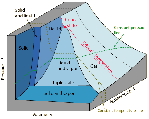
We have seen 3 different equations of state that describe different phases, but real substances are more complex and generally cannot be described with a single equation of state, requiring interpolation between different equations of state for different phases, often from empirical data. These are known as $P$-$v$-$T$ surfaces and are 3-dimensional surfaces, as shown below:
Source: HyperPhysics
A non-elementary discussion of $P$-$v$-$T$ surfaces is beyond the scope of this guide. However, we will highlight two notable features that one finds on them which is not described by simple equations of state. First, it is possible for a substance to be solid, liquid, and gas at the same time(!) which is known as a triple state, and marked by a line on a $P$-$v$-$T$ surface. It is also possible at certain pressures and temperatures for a gas to directly transition to a solid (sublimation), which we commonly observe in solid carbon dioxide (dry ice).
State variables and exact differentials
The mathematical basis for state variables comes from multivariable calculus, which we will take a moment to revisit. Consider an arbitrary function of two variables $z = z(x, y)$ (in thermodynamics this is typically the equation of state). The total differential $dz$ may be expressed as:
$$ dz = \frac{\partial z}{\partial x} dx + \frac{\partial z}{\partial y}dy $$
We may also rewrite this as:
$$ dz = A dx + B dy, \quad A \equiv \frac{\partial z}{\partial x}, \quad B \equiv \frac{\partial z}{\partial y} $$
Now, if the above is true, it must also be true that:
$$ \left( \frac{\partial A}{\partial y} \right)_{x} = \left( \frac{\partial B}{\partial x} \right)_{y} $$
Where the subscript $x$ means “with $x$ held constant” and the subscript $y$ means “with $y$ held constant”. This becomes clear if we substitute in the definitions of $A$ and $B$, since:
$$ \begin{align*} \left( \frac{\partial A}{\partial y} \right)_{x} &= \left( \frac{\partial}{\partial y}\left[ \frac{\partial z}{\partial x} \right] \right)_{x} = \frac{\partial^2 z}{\partial y \partial x} \\ \left( \frac{\partial B}{\partial x} \right)_{y} &= \left( \frac{\partial}{\partial x} \left[ \frac{\partial z}{\partial y} \right] \right)_{y} = \frac{\partial^2 z}{\partial x \partial y} \end{align*} $$
Since we know that mixed 2nd (partial) derivatives are equal, one has:
$$ \frac{\partial^2 z}{\partial y \partial x} = \frac{\partial^2 z}{\partial x \partial y} \implies \left( \frac{\partial A}{\partial y} \right)_{x} = \left( \frac{\partial B}{\partial x} \right)_{y} $$
We thus say that $dz$ is an exact differential as a result, and state variables in thermodynamics must be expressible as exact differentials. State variables in thermodynamics are not just expressible as exact differentials — any function of state variables is also a state variable, making it an exact differential too!
As an example, let $v = v(T, P)$, where $v$ is the specific volume, $T$ is the temperature, and $P$ is the pressure. Since volume (and therefore specific volume) is a state variable, we may express it as an exact differential $dv$, where $dv$ is given by:
$$ dv = \left( \frac{\partial v}{\partial T} \right)_{P} dT + \left( \frac{\partial v}{dP} \right)_{T} dP $$
Where the subscripts $P$ and $T$ indicate that pressure and temperature should respectively be held constant when taking the derivative. It is common to rewrite $dv$ in the form:
$$ dv = v \beta dT - v \kappa dP $$
Where $\beta$ is the expansivity, $\kappa$ is compressibility, and where:
$$ \beta \equiv \frac{1}{v} \left( \frac{\partial v}{\partial T} \right)_{P}, \kappa \equiv -\frac{1}{v} \left( \frac{\partial v}{\partial P} \right)_{T} $$
For an ideal gas, we can rearrange the ideal gas law $Pv = RT$ into $v = RT/P$. From there, we find that:
$$ \beta = \frac{1}{T}, \quad \kappa = \frac{1}{P} \quad \text{(ideal gas)} $$
For a liquid or solid, where we assume that the volume is roughly constant ($v \approx v_0 = \text{const.}$) and where we consider discrete changes in temperature ($\Delta T$) and pressure ($\Delta P$), the change in specific volume may then be expressed as:
$$ \Delta v = v_0(\beta \Delta T - \kappa \Delta P) $$
A key property of exact differentials is that they are path-independent for any given path through their state space. This is due to the gradient theorem, which states that for an exact differential $dz$, its line integral between points $A$ and $B$ in the state space is given by:
$$ \int_{A}^B dz = z(B) - z(A) $$
In thermodynamics, this is important because it means that as long as we are dealing with state variables, we can decompose arbitrarily-complex processes as a sequence of simpler processes (typically isothermal, isobaric, isochoric, and/or adiabatic processes) which together have the same initial and final states as the more complex process under examination. Path independence means that the simpler sequence of processes is mathematically equivalent to the complex single process. Moreover, it means that for a reversible process, there is no net change in the state variable if the process is subsequently reversed:
$$ \oint dz = \int_{A}^B dz + \int_{B}^A dz = 0 $$
Exact differentials satisfy some special relations, which are useful for solving problems. First, they satisfy the reciprocity relation:
$$ \left( \frac{\partial z}{\partial x} \right)_{y} = \left( \frac{\partial x}{\partial z} \right)_{y}^{-1} $$
Second, they satisfy the cyclic relation:
$$ \left( \frac{\partial x}{\partial y} \right)_{z} \left( \frac{\partial y}{\partial z} \right)_{x} \left( \frac{\partial z}{\partial x} \right)_{y} = -1 $$
Units in thermodynamics
In this guide we will primarily be using SI units, where:
- Pressure is in units of Pascals (denoted $\pu{Pa}$), where $\pu{1 Pa} = \pu{1 N/m^2}$
- Temperature is in units of Kelvin (denoted $\pu{K}$)
- Volume is in units of liters (denoted $\pu{L}$) or cubic meters (denoted $\pu{m^3}$) or cubic centimeters (denoted $\pu{cm^3}$). Note that $\pu{1 L} = \pu{1000 cm^3} = \pu{0.001 m^3}$
However, we will also be using some non-SI units. For instance, we will use the Celsius scale and Fahrenheit scale for temperature where appropriate. We may convert between Celsius and Kelvin using the formula:
$$ T[{}^\circ\text{C}] = T[\pu{K}] - 273.15 $$
Where $T[{}^\circ\text{C}]$ is the temperature in degrees Celsius and $T[\pu{K}]$ is the temperature in Kelvin. We may also convert temperature between Celsius and Fahrenheit as follows:
$$ \begin{align*} T[{}^\circ\text{F}] &= \frac{9}{5} T[{}^\circ\text{C}] + 32 \\ T[{}^\circ\text{C}] &= \frac{5}{9} (T[{}^\circ\text{F}] - 32) \end{align*} $$
Where $9/5 = 1.8 \approx 2$, hence a rule of thumb when roughly converting between Fahrenheit and Celsius is to double the temperature in Celsius, then add 32. A useful table for common conversion values can be found on this PDF.
Note: In certain fields of engineering, the antiquated Rankine scale is used as an alternative scale for measuring temperature, although it is rarely used nowadays. We will thus not use it in this guide. However, for interested readers, the Rankine scale is defined such that 1 Rankine (symbol ${}^\circ R$) is equal to five-ninths of a Kelvin, that is, $\pu{1 {}^\circ R} = \frac{5}{9}\pu{K}$.
We will also use other pressure units. One common unit for pressure is the standard atmosphere (symbol $\pu{atm}$), where $\pu{1 atm} = \pu{101325 Pa} \approx \pu{10^5 Pa}$ and is approximately equal to Earth’s atmospheric pressure at sea level. Another unit is the torr, where $\pu{1 atm} = \pu{760 torr}$. In medicine, a common alternative pressure unit is the millimeter of mercury (symbol $\pu{mmHg}$) which is approximately equal to 1 torr. A variety of other pressure units can be found on this table on Wikipedia.
The zeroeth law of thermodynamics
Thermodynamic systems, no matter their behavior or constituents, obey several fundamental laws. We will start with the zeroeth law of thermodynamics, which was discovered empirically. It states that if we have three isolated systems $A, B, C$, where system $A$ is in thermal equilibrium with system $B$ and system $B$ is in thermal equilibrium with system $C$, then system $A$ must be in equilibrium with system $C$.
This conclusion may seem trivial, but it actually has important consequences. First, it is the physical principle that permits thermometers to be possible, because one cannot measure the temperature of a system directly; we can only ever measure the temperature of another system that is at thermal equilibrium with the system we’re studying. Indeed, temperature is only defined thanks to the zeroeth law! Second, and more importantly, it sets a limit on how “cold” something can be. This is because it implies that to cool a system, you must allow it to achieve thermal equilibrium with a colder system. However, this can only go down to a certain point, below which you simply cannot go colder. This is known as absolute zero and is the theoretically coldest temperature possible, which is defined to be at zero Kelvin or $\pu{-273.15^\circ C}$.
Types of processes
Physically, a thermodynamic process is a change in a system, where pressure, volume, and/or temperature change. Mathematically, a thermodynamic process is a transition between two points in the thermodynamic state space. We can characterize processes using the following classifications:
| Type | Defining characteristics |
|---|---|
| Reversible process | Process in which there is no energy dissipation, allowing it to be perfectly reversed |
| Irreversible process | Process in which there is unavoidable energy dissipation, making it impossible to perfectly reverse |
| Cyclic process | Combination of several processes that repeat in an infinite cycle in the form $A \to B \to C \to A \to B \to C \to \dots$ |
| Diathermal process | No mass transfer but there is heat transfer |
| Adiabatic process | No heat transfer is present |
| Isobaric process | Process occurs at constant pressure ($dP = 0$) |
| Isothermal process | Process occurs at constant temperature ($dT = 0$) |
| Isochoric process | Process occurs at constant volume ($dV = 0$) |
| Quasi-static process | Process that happens slow enough that a system remains in thermodynamic equilibrium. All reversible processes and some irreversible processes are quasi-static. |
Note: In physical nature, all processes are ultimately irreversible, but can be approximated by ideal, reversible processes, or at least a sequence of reversible processes. We will later show that this is an inevitable consequence of the second law of thermodynamics
Note for the advanced reader: The term adiabatic is also used loosely in other fields of physics; the well-known adiabatic approximation in quantum mechanics does not strictly correspond to thermodynamically-adiabatic processes, but rather is a general form of quasi-static approximation.
There is an important link between the physical and mathematical descriptions of a process. Specifically, isobaric processes correspond mathematically to isobars of the equation of state, while isothoric processes similarly correspond to isothors and isothermal processes correspond to isotherms.
Finally, the notion of a quasi-static process is essential, because (as we mentioned earlier) (classical) thermodynamics only applies for systems in thermal equilibrium. This means that we can only analyze processes that can be described as a set of (potentially-infinite) equilibrium states. An explosive reaction or a rapid compression of a piston is not quasi-static and therefore cannot be formally described using thermodynamics.
Show table of contents Back to all notes